Performance¶

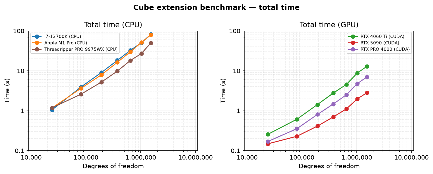
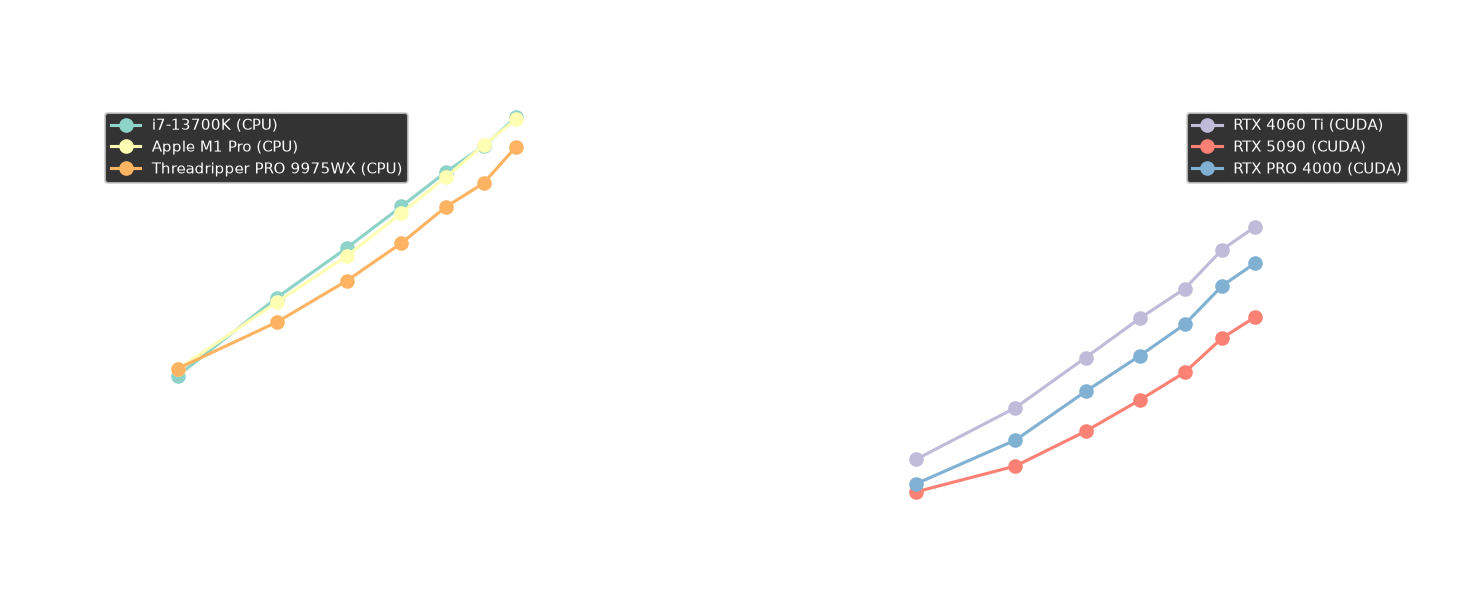
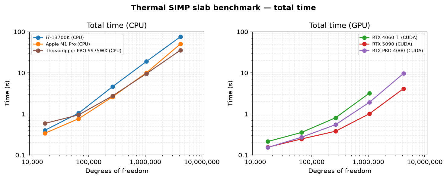
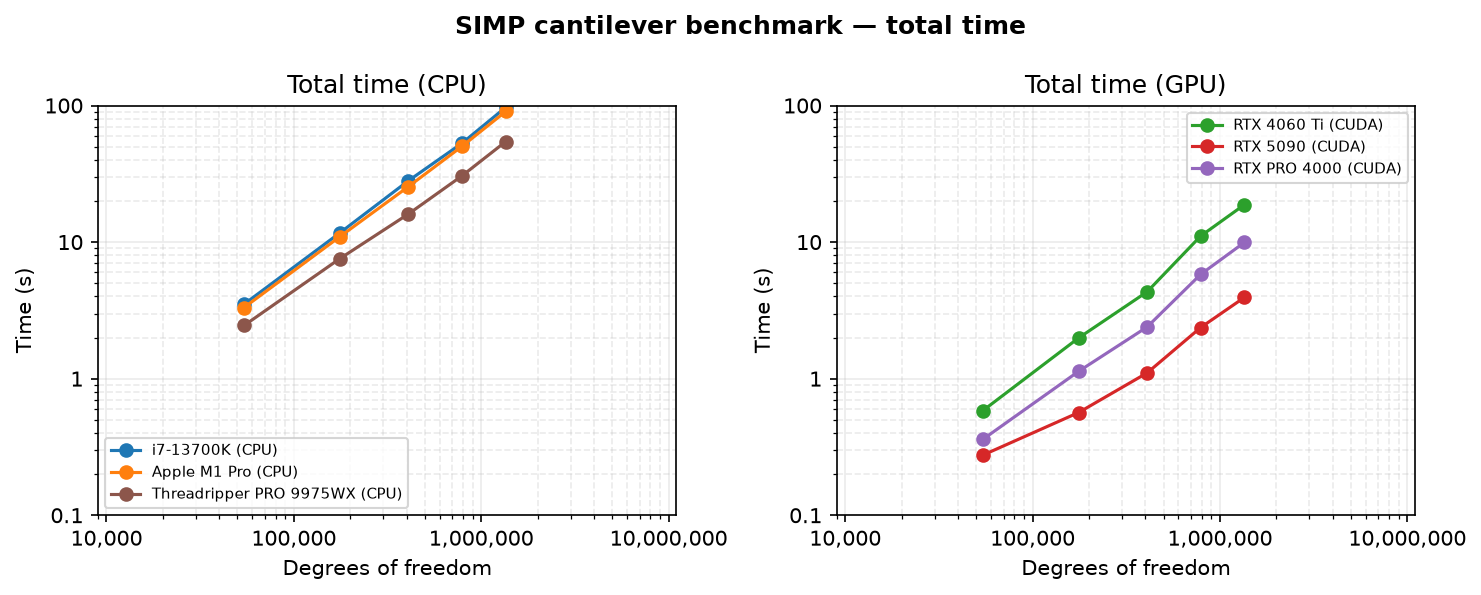
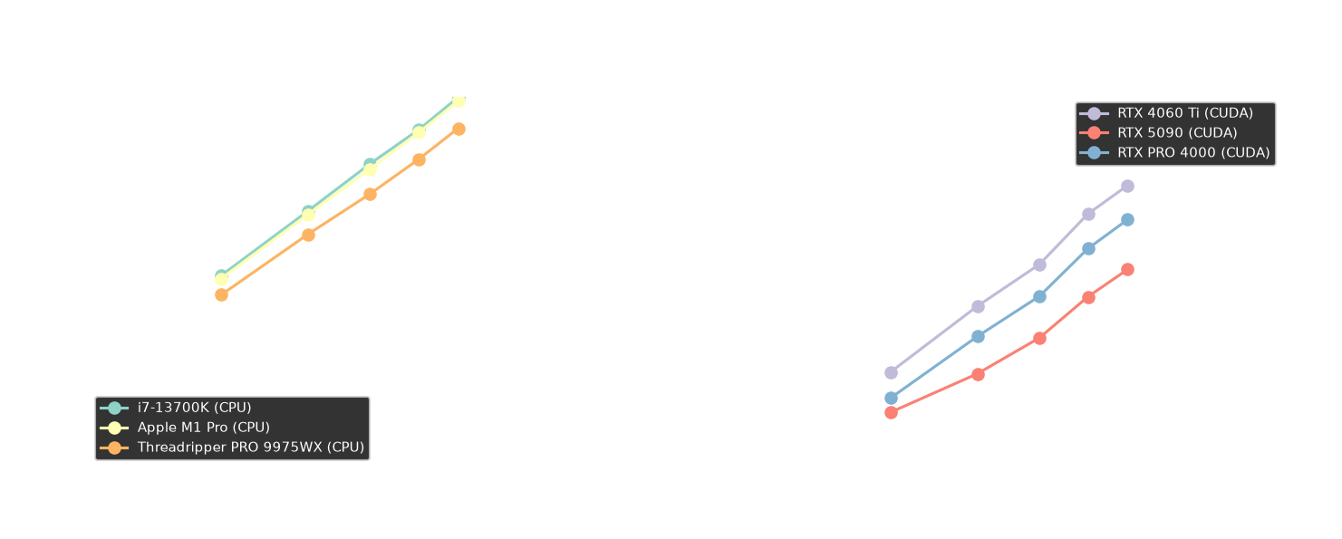
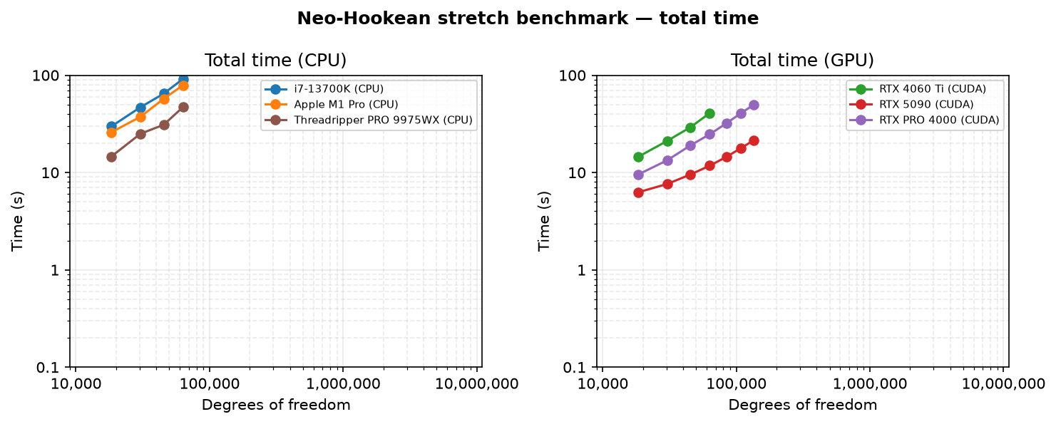
Scaling behavior of torch-fem on four benchmark problems across several machines. The plotted time is the total of three phases, each of which is recorded separately in the result files:

1. Setup: mostly computing the sparsity pattern.

2. Forward solve: assembly and sparse linear solve.

3. Backward solve: reverse-mode AD through the solve via autograd.

Cube extension¶

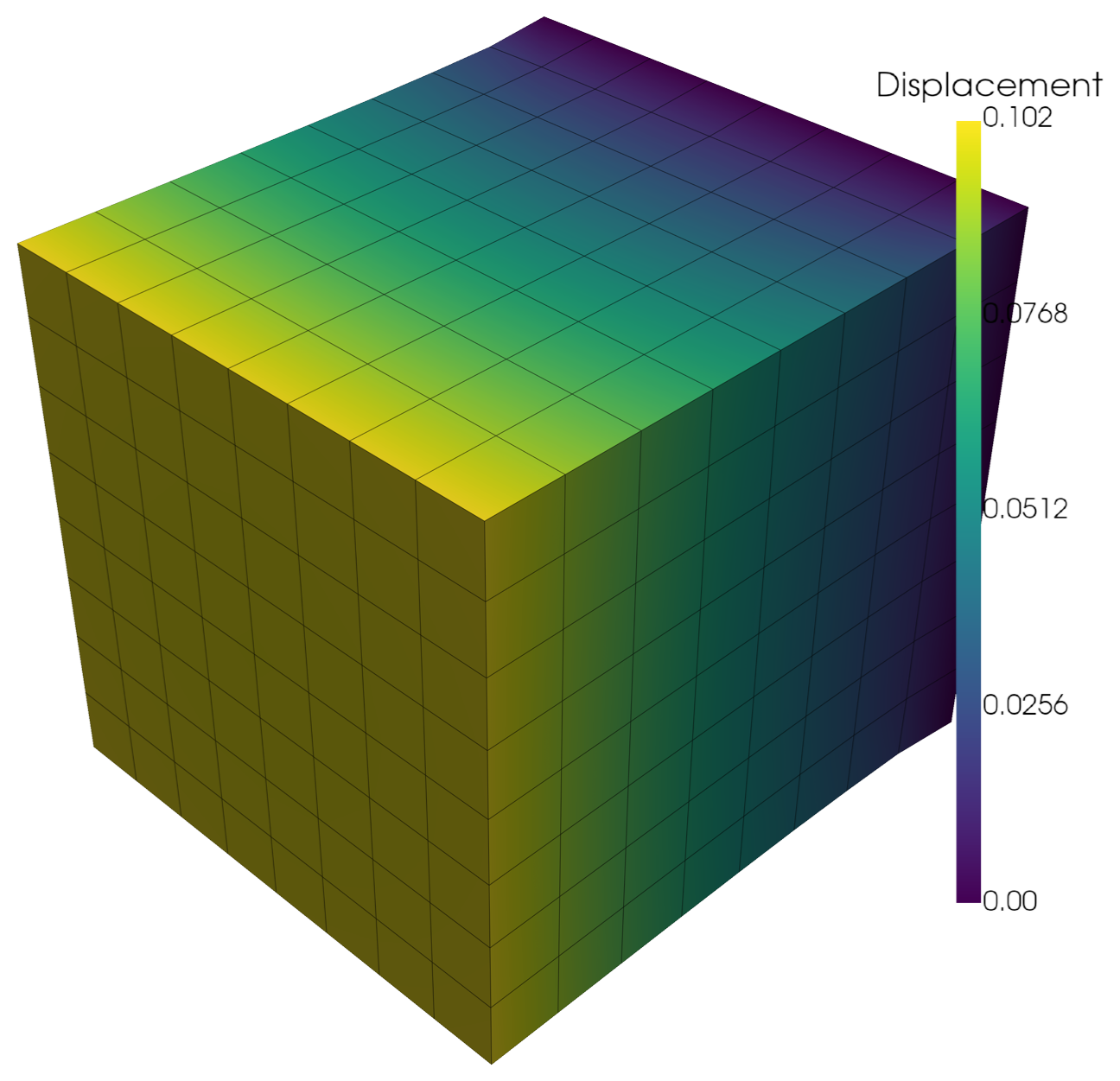
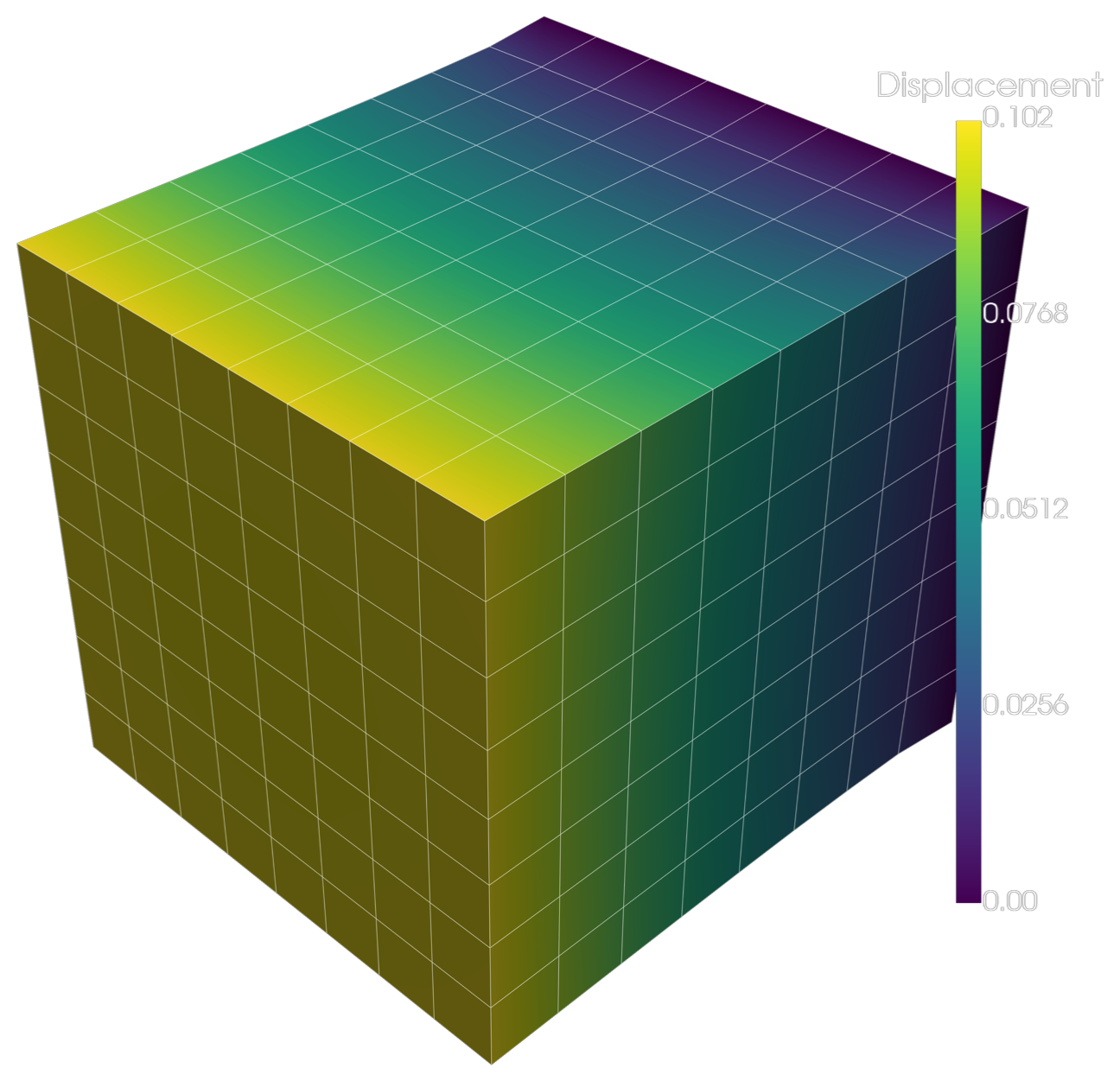
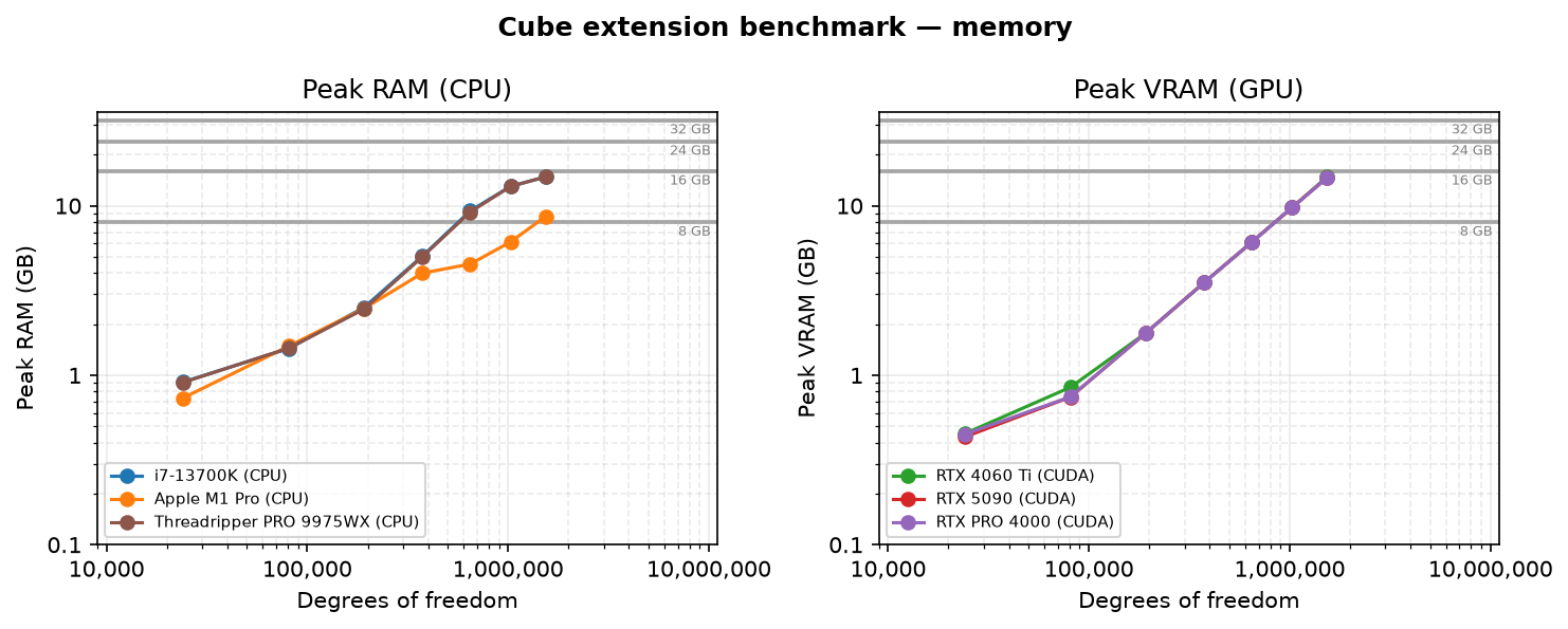
A unit cube from linear hexahedra with \(N\) nodes along each edge (\(3N^3\) degrees of freedom) in isotropic linear elasticity (\(E = 1000\), \(\nu = 0.3\)), clamped at \(x = 0\) and pulled to \(u_x = 0.1\) at \(x = 1\). The backward pass takes the gradient of u.sum() with respect to the nodal forces.

Thermal SIMP slab¶

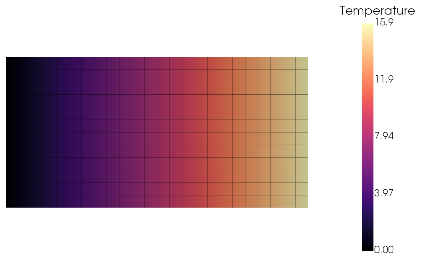
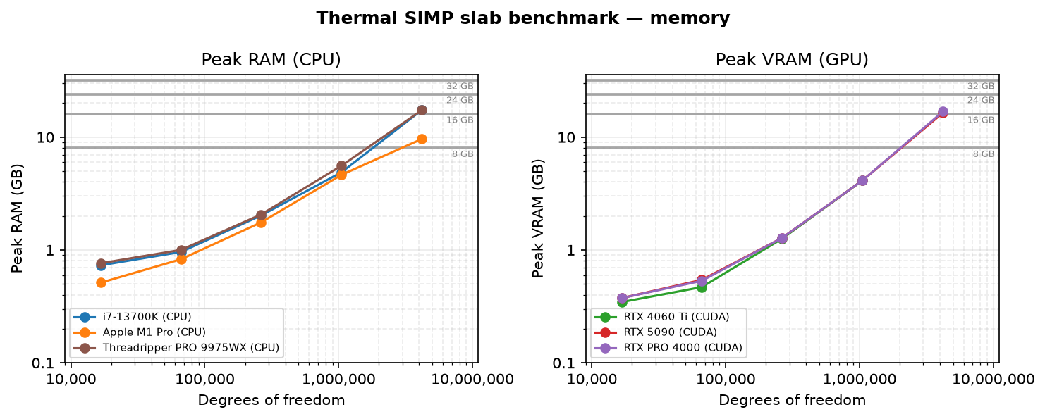
A quasi-2D slab on \([0,2] \times [0,1]\), one layer of cubic hexahedra deep and \(N\) elements along the long edge, carrying SIMP-penalized conductivity \(k(\rho) = k_\text{min} + (k_\text{max} - k_\text{min})\rho^3\) at uniform \(\rho = 0.5\). It is cold at \(x = 0\) and heated by a uniform flux at \(x = 2\); the backward pass is the adjoint sensitivity of the thermal compliance with respect to the per-element densities. This mirrors the thermal-mesh problem of the mosaic benchmark suite.

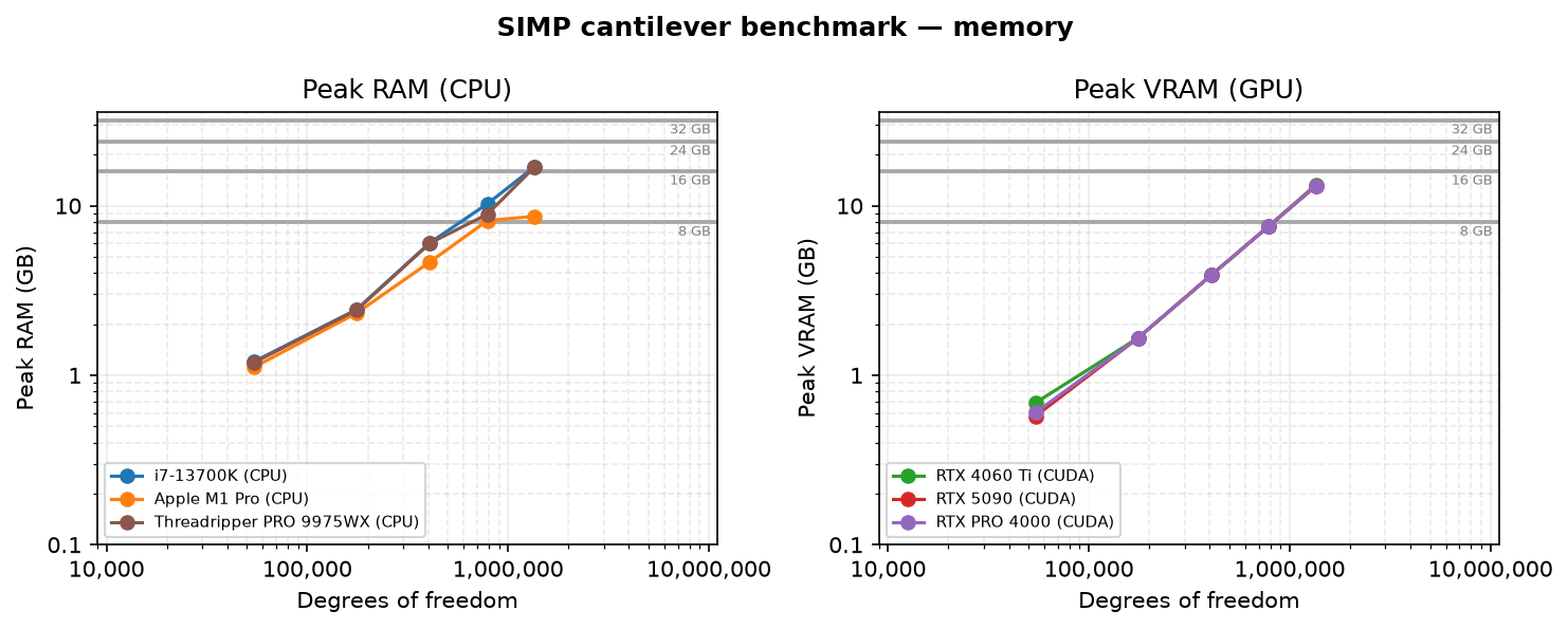
SIMP cantilever¶

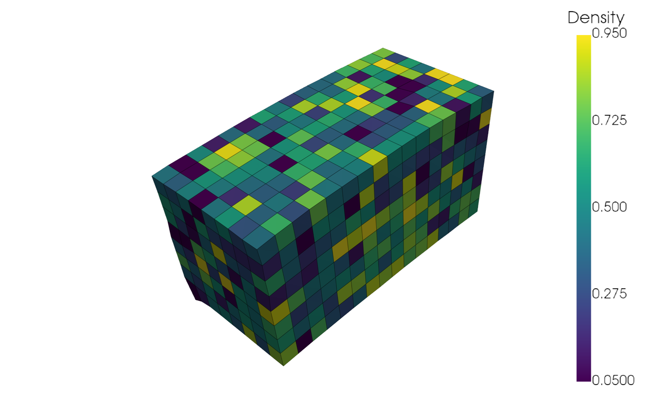
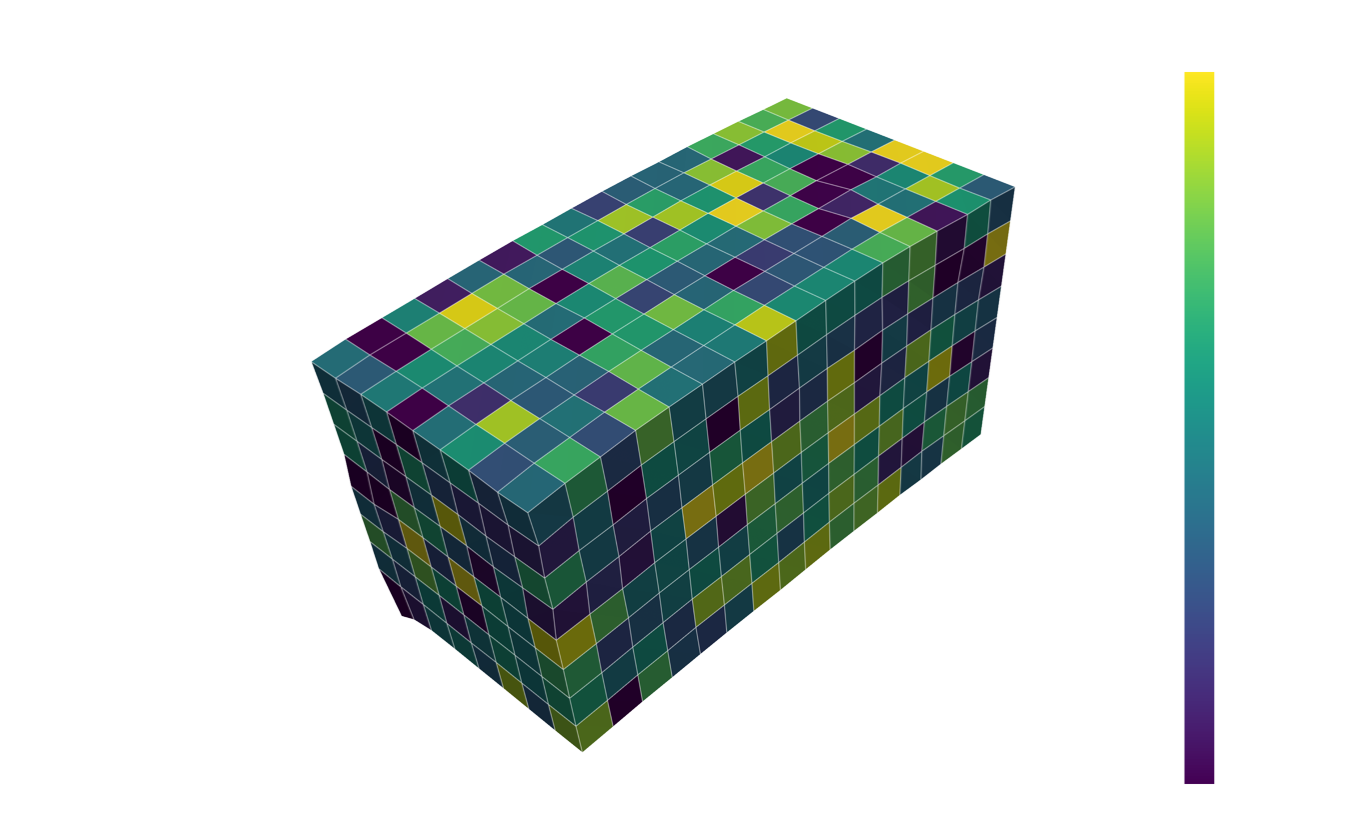
A cantilever on \([0,2] \times [0,1] \times [0,1]\) of \(2N \times N \times N\) cubic hexahedra, carrying SIMP-penalized stiffness \(E(\rho) = E_\text{min} + (E_\text{max} - E_\text{min})\rho^3\) at \(E_\text{max} = 70{,}000\). It is clamped at \(x = 0\) and pulled down by a uniform traction at \(x = 2\); the backward pass is the adjoint sensitivity of the compliance \(C = \mathbf{F}^\top \mathbf{u}\) with respect to the per-element densities. Those are random, \(\rho \sim \mathcal{N}(0.5, 0.3)\) clipped to \([0.05, 0.95]\), which spreads element stiffness over a factor of 762 and roughly doubles the iteration count of the preconditioned solver. This mirrors the structural-mesh problem of the mosaic benchmark suite and reproduces its published compliances to a relative error of \(10^{-7}\).

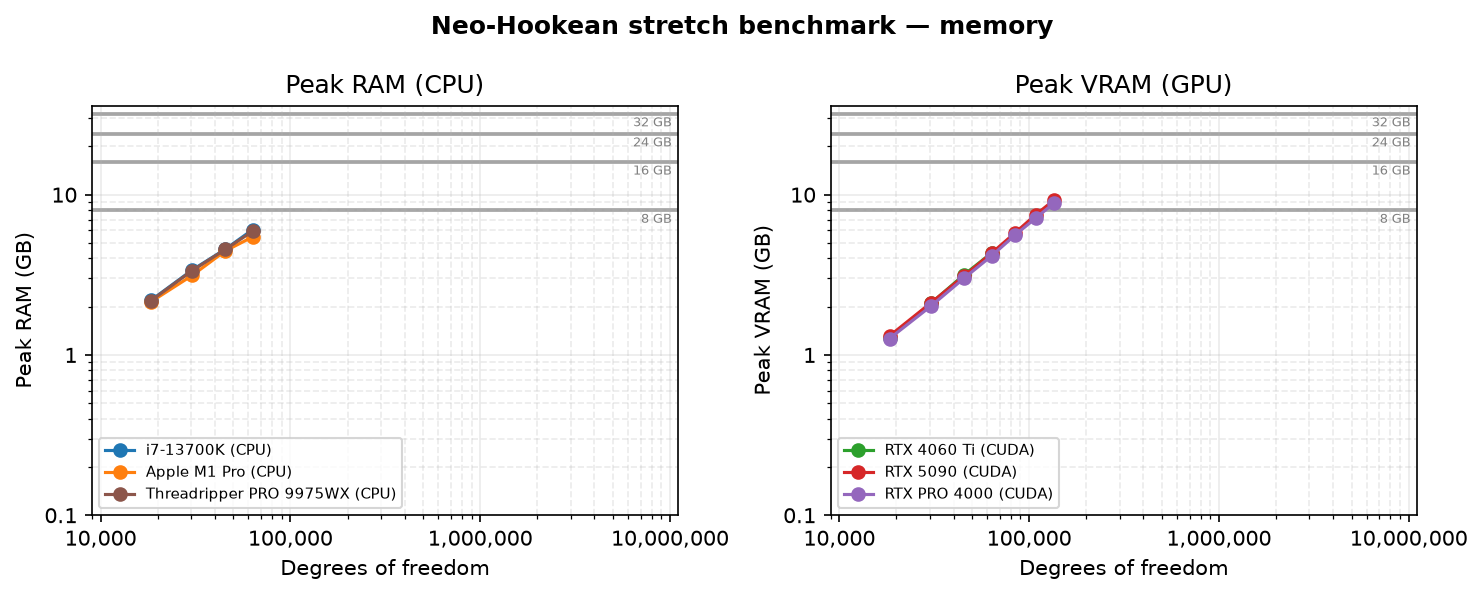
Neo-Hookean stretch¶

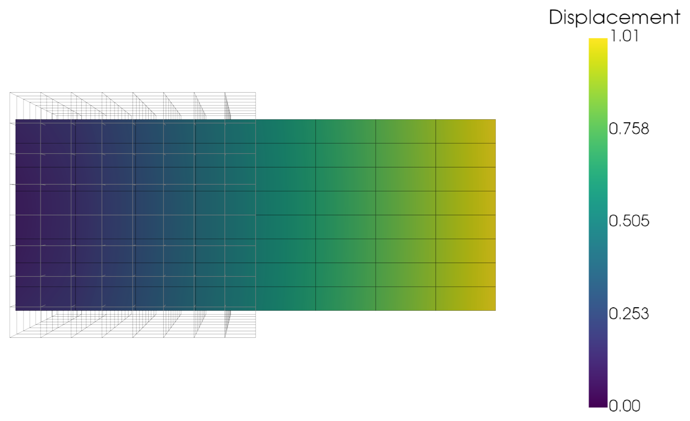
A box of Neo-Hookean material stretched to ten times its length in 10 increments, geometric in the stretch, with full Newton iterations, mirroring the large stretch example. Only \(y\) and \(z\) are refined, with \(N\) nodes each over four cubic elements along the stretch direction (\(15N^2\) degrees of freedom), since the solution is homogeneous and a longer stretch drives the tangent indefinite. The forward solution matches the analytical uniaxial response; the backward pass is the adjoint of the total reaction force with respect to the Lamé parameters, as used in material calibration.

Reproducing the results¶

The scripts live in benchmarks/ at the repository root.

1. Run the benchmark:

# All benchmarks on CPU (default)
python benchmarks/run.py

# Just the cube benchmark on CUDA
python benchmarks/run.py -problem cube -device cuda --label rtx5090_cuda --hardware "RTX 5090"

The label identifies the machine; results are written to benchmarks/results/<problem>_<label>.json.

2. Regenerate the plots:

python benchmarks/plot.py

This reads all JSON files in benchmarks/results/, groups them by problem, and writes the timing, backward, and RAM plots to docs/images/benchmark/<problem>_*.png.