In this chapter, we focus on the optimization of discrete truss
structures. A general procedure to solve such problems involves the
following steps:
Definition of the truss with all nodes, elements, material
properties, constraints and initial design choice
Solution of unknown displacements for each node in the truss
given the current design
Evaluation of the objective function and its gradients w.r.t. the
design variables
Approximation of the problem with MMA at the current design
point
Solution of the approximated dual problem to find the next design
point
Repetition of steps 2,3,4 and 5 until a maximum of iterations is
reached or until there is no improvement of the objective function any
more
Learning Objectives
After studying this chapter and finishing the exercise, you should be
able to
define optimization problems to minimize compliance of
two-dimensional trusses with a volume constraint
explain properties of the aforementioned optimization
problem
employ MMA to solve two-dimensional truss optimization
problems
6.1 Size Optimization
One possible objective in truss optimization is the search for the
cross sectional areas \(\mathbf{a}\)
resulting in the stiffest truss. The corresponding objective function
could be simply the displacement at a specific node or a global
displacement measure \(\mathbf{u} (\mathbf{a})
\cdot \mathbf{u} (\mathbf{a})\). However, we choose to minimize
the compliance \(C: \mathcal{R}^{M}
\rightarrow \mathcal{R}\) defined as \[C(\mathbf{a}) = \mathbf{f} \cdot
\mathbf{u}(\mathbf{a}){\qquad(6.1)}\] of the truss instead. The
minimal compliance results also in the stiffest truss, but this
formulation is preferred over the pure displacement formulation, because
\(C(\mathbf{a})\) is convex (Svanberg 1985). The
convexity is proven by showing that the Hessian \(\nabla^2 C(\mathbf{a})\) is positive
semi-definite, a property that is inherited from the positive
semi-definiteness of \(\mathbf{K}(\mathbf{a})\) (see Chapter 5.2.1
in (Christensen and
Klarbring 2008) for details).
We employ box constraints \(\mathcal{A}\) on the upper and lower limit
of the design variables. The upper limit \(\mathbf{a}^+\) could be a manufacturing
constraint that prevents very thick elements. The lower limit \(\mathbf{a}^-\) should be larger than \(0\) to prevent deletion of truss elements.
If the cross sectional area of all elements connected to a node would
become \(0\), i.e. all trusses are
deleted, the displacement of that node would be undetermined and the
stiffness matrix would become singular. In this chapter, we prevent this
by demanding \(a_j^- > 0\).
A typical inequality constraint is a volume constraint for the total
truss volume used in the assembly. If we would not have a volume
constraint, the optimization would predict a trivial solution with all
cross sections at their maximum area. However, we are interested in
solutions that put a limited material resource to its best use and thus
limit the total volume to be \[\mathbf{a}
\cdot \mathbf{l} \le V_0{\qquad(6.2)}\] where \(V_0\) describes the maximum volume used in
the design In order to find a solution at all, we must obviously choose
\(V_0 \ge \mathbf{a}^- \cdot
\mathbf{l}\), otherwise it would be impossible to find any \(\mathbf{a}\) fulfilling the constraint.
In conclusion, the size optimization problem for a stiff truss with
limited volume may be noted as follows:
The objective function \(C(\mathbf{a})\) is convex, the inequality
constraint \(\mathbf{a} \cdot \mathbf{l} -
V_0\) is convex, and the set \(\mathcal{A}\) is compact and convex.
Therefore, finding a KKT point is equivalent to finding the global
unique solution of the problem. We can denote the Lagrangian \[\mathcal{L}(\mathbf{a}, \mu) = C(\mathbf{a}) +
\mu \left( \mathbf{a} \cdot \mathbf{l} - V_0
\right){\qquad(6.4)}\] and need to compute the gradient \(\frac{\partial \mathcal{L}}{\partial a_j}\)
to solve the optimization problem. It is \[\frac{\partial \mathcal{L} (\mathbf{a},
\mu)}{\partial a_j}
= \frac{\partial C (\mathbf{a})}{\partial a_j} + \mu l_j
= \mathbf{f} \cdot \frac{\partial \mathbf{u} (\mathbf{a})}{\partial
a_j} + \mu l_j,
\label{eq:lagrange_truss_problem}{\qquad(6.5)}\] where the
gradient \(\frac{\partial \mathbf{u}
(\mathbf{a})}{\partial a_j}\) remains to be determined. It can be
obtained by differentiating Equation w.r.t \(\mathbf{a}\)\[\begin{aligned}
\frac{\partial}{\partial a_j} \mathbf{f} &=
\frac{\partial}{\partial a_j} \left( \mathbf{K} (\mathbf{a}) \cdot
\mathbf{u} (\mathbf{a}) \right) {\qquad(6.6)}\\
0 &= \frac{\partial \mathbf{K} (\mathbf{a})}{\partial a_j}
\cdot \mathbf{u} (\mathbf{a}) + \mathbf{K} (\mathbf{a}) \cdot
\frac{\partial \mathbf{u} (\mathbf{a})}{\partial a_j}
{\qquad(6.7)}\end{aligned}\] and rearranging the terms to yield
\[\frac{\partial \mathbf{u}
(\mathbf{a})}{\partial a_j} = - \mathbf{K}^{-1}(\mathbf{a}) \cdot
\frac{\partial \mathbf{K} (\mathbf{a})}{\partial a_j} \cdot \mathbf{u}
(\mathbf{a}).{\qquad(6.8)}\] Substituting this expression into
the previous Equation 6.5 gives
us the sensitivity of the compliance with respect to the design
variables \[\begin{aligned}
\frac{\partial C (\mathbf{a})}{\partial a_j}
&= - \mathbf{f} \cdot \mathbf{K}^{-1}(\mathbf{a}) \cdot
\frac{\partial \mathbf{K} (\mathbf{a})}{\partial a_j} \cdot \mathbf{u}
(\mathbf{a}) {\qquad(6.9)}\\
&= - \mathbf{u} (\mathbf{a}) \cdot \frac{\partial \mathbf{K}
(\mathbf{a})}{\partial a_j} \cdot \mathbf{u}
(\mathbf{a}) {\qquad(6.10)}\\
&= - \mathbf{u}_j (\mathbf{a}) \cdot \frac{\partial
\mathbf{k}_j(a_j)}{\partial a_j} \cdot \mathbf{u}_j
(\mathbf{a}) {\qquad(6.11)}\\
&= - \mathbf{u}_j (\mathbf{a}) \cdot \mathbf{k}^0_j \cdot
\mathbf{u}_j (\mathbf{a}) {\qquad(6.12)}\\
&= - 2 w_j (\mathbf{a})
\label{eq:compliance_sensitivity}
{\qquad(6.13)}\end{aligned}\] with \[\mathbf{k}_j^0 = \frac{E}{l_j}
\begin{pmatrix}
\cos{\phi}^2 & \cos{\phi}\sin{\phi} & -\cos{\phi}^2 &
-\cos{\phi}\sin{\phi} \\
\cos{\phi}\sin{\phi} & \sin{\phi}^2 & -\cos{\phi}\sin{\phi}
& -\sin{\phi}^2 \\
-\cos{\phi}^2 & -\cos{\phi}\sin{\phi} & \cos{\phi}^2
&\cos{\phi}\sin{\phi} \\
-\cos{\phi}\sin{\phi} & -\sin{\phi}^2 & \cos{\phi}\sin{\phi}
& \sin{\phi}^2 \\
\end{pmatrix}{\qquad(6.14)}\] and the strain energy density
in each element \[w_j = \frac{1}{2}
\mathbf{u}_j (\mathbf{a}) \cdot \mathbf{k}^0_j \cdot \mathbf{u}_j
(\mathbf{a}).
\label{eq:element_strain_energy}{\qquad(6.15)}\] The strain
energy density is always greater or equal to zero due to the positive
semi-definiteness of \(\mathbf{k}^0_j\). What we have just done is
called a sensitivity analysis - we obtained an expression of
how much a change of variable \(a_j\)
contributes to the change of the objective function \(\frac{\partial C (\mathbf{a})}{\partial
a_j}\). It is very valuable to have an analytical expression of
the sensitivity, as solving it numerically via finite differences causes
a high computational cost and loss in precision. Finally, the gradient
of the Lagrangian becomes \[\frac{\partial
\mathcal{L} (\mathbf{a}, \mu)}{\partial a_j}
= - 2 w_j (\mathbf{a}) + \mu l_j
\label{eq:lagrange_sensitivity}{\qquad(6.16)}\]
If we could solve this expression for \(\mathbf{a}^*(\mu)\) at the stationary point
of the Lagrangian, we could use Lagrangian duality to compute the
solution easily. Unfortunately, the solution is not easy, as \(w_j\) depends on the global design \(\mathbf{a}\) and not just on the design
variable in its element \(a_j\). For
this reason, we will use MMA to solve the problem.
Example: Fully stressed design
We can still learn something about the solution if we consider Equation
6.15. If we substitute it in
Equation 6.16, we can write \[\frac{\partial \mathcal{L} (\mathbf{a},
\mu)}{\partial a_j} = - \frac{\sigma^2_j}{E} l_j + \mu
l_j{\qquad(6.17)}\] and conclude that for an optimal point \(\mathbf{a}^- < \mathbf{a}^* <
\mathbf{a}^+\) with \(\mu^*>0\), i.e. the maximum volume \(V_0\) is used and box constraints are not
reached, all stress magnitudes are identical with \[\sigma_j = \pm \sqrt{\mu^*
E}.{\qquad(6.18)}\]
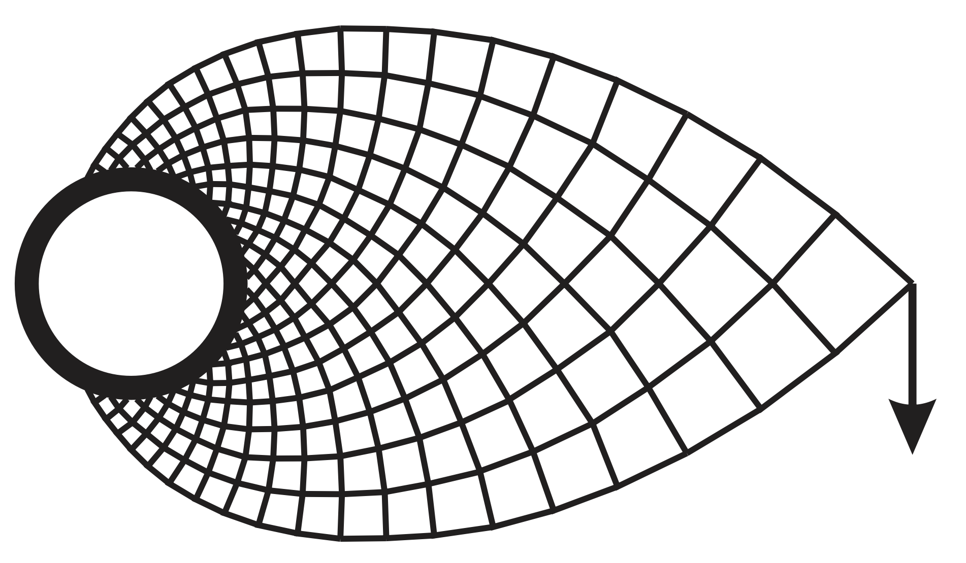
This is called a fully stressed design and is related to a
theorem by Australian engineer A.G.M. Michell published in 1904 (Michell 1904). The
theorem states that elements of an optimal truss structure lie along the
principal directions of a virtual stress field, such that all of them
experience an equal stress magnitude (Arora et al. 2019). An example for a
Michell truss structure is given in the following picture (Picelli 2015). All
truss elements in this design experience the same stress magnitude
(either in compression or in tension).
The problem in Equation 6.3 is
convex, but it is not separable and explicit, because we cannot find an
explicit expression for \(\mathbf{a}^*(\mu)\) at the stationary point
of the Lagrangian. Therefore we linearize the problem using MMA in \(1/(a_j-L_j^k)\). The linearization of the
objective function becomes \[\begin{aligned}
\tilde{C}(\mathbf{a}) &= C(\mathbf{a}^k) + \sum_j \frac{\partial
C}{\partial a_j}(\mathbf{a}^k) (a^k_j-L^k_j) - \sum_j \frac{\partial
C}{\partial a_j}(\mathbf{a}^k)
\frac{(a^k_j-L^k_j)^2}{a_j-L^k_j}{\qquad(6.19)}\\
&=C(\mathbf{a}^k)
- \sum_j 2w_j (\mathbf{a}^k) (a^k_j-L^k_j)
+ \sum_j 2w_j (\mathbf{a}^k)
\frac{(a^k_j-L^k_j)^2}{a_j-L^k_j}.
{\qquad(6.20)}\end{aligned}\] Note that this is a linearization
using lower asymptotes only, because \[\frac{\partial C }{\partial a_j}(\mathbf{a}^k) =
- 2 w_j (\mathbf{a}^k) < 0 \quad \forall
\mathbf{a}^k{\qquad(6.21)}\] and thus all terms in Equations and
involving \(p_j^k\) vanish. The
approximated optimization problem becomes \[\begin{aligned}
\min_{\mathbf{a}} \quad & \tilde{C}
(\mathbf{a}){\qquad(6.22)}\\
\textrm{s.t.} \quad & \mathbf{a} \cdot \mathbf{l} - V_0 \le
0 {\qquad(6.23)}\\
& \tilde{\mathbf{a}}^{-,k} \le
\mathbf{a} \le \mathbf{a}^+{\qquad(6.24)}\\
{\qquad(6.25)}\end{aligned}\] with lower move limits \(\tilde{\mathbf{a}}^{-,k} = \max(\mathbf{a}^-, 0.9
\mathbf{L}^k + 0.1 \mathbf{a}^k)\) preventing division by zero.
The constraint is already linear and thus we do not approximate it.
The Lagrangian of the approximated problem is \[\mathcal{L}(\mathbf{a}, \mu) =
\tilde{C}(\mathbf{a}) + \mu \left( \mathbf{a} \cdot \mathbf{l} - V_0
\right){\qquad(6.26)}\] is separable with \[\begin{split}
\mathcal{L}(\mathbf{a}, \mu) &= \underbrace{C(\mathbf{a}^k)
- \sum_j 2w_j (\mathbf{a}^k) (a^k_j-L^k_j) - \mu V_0}_{\mathcal{L}^0} \\
&+ \sum_j \underbrace{\left(2 w_j (\mathbf{a}^k)
\frac{(a^k_j-L^k_j)^2}{a_j-L^k_j} + \mu a_j l_j
\right)}_{\mathcal{L}_j (a_j)}.
\end{split}{\qquad(6.27)}\] We want to find an explicit
expression for \(\mathbf{a}^*(\mu)\).
Therefore we compute the stationary point of the Lagrangian \[\frac{\partial \mathcal{L}_j}{\partial a_j} = -2
w_j (\mathbf{a}^k)
\frac{(a^k_j-L^k_j)^2}{(\hat{a}_j-L^k_j)^2} + \mu l_j =
0{\qquad(6.28)}\] and rearrange the equation to find \[\hat{a}_j(\mu) = L_j^k + \sqrt{\frac{2 w_j
(\mathbf{a}^k)
(L^k_j-a^k_j)^2}{\mu l_j}}.{\qquad(6.29)}\] We simply clamp
this result with box constraints to obtain the explicit relation \[\mathbf{a}^* (\mu) =
\textrm{clamp}\left(\hat{\mathbf{a}}(\mu), \tilde{\mathbf{a}}^{-,k},
\mathbf{a}^+\right).{\qquad(6.30)}\] Finally we can plug this
result in the Lagrangian to get the dual function \[\underline{\mathcal{L}}(\mu) =
\mathcal{L}(\mathbf{a}^* (\mu), \mu){\qquad(6.31)}\] and solve
\[\max_{\mu}
\underline{\mathcal{L}}(\mu){\qquad(6.32)}\] for \(\mu^*>0\). This solution procedure is
simple - the dual Lagrangian depends only on one variable and the
problem is concave. We can use a gradient descent method to solve it
quickly and utilize this analytical expression for the gradient \[\frac{\partial \underline{\mathcal{L}}}{\partial
\mu}(\mu) = \mathbf{a}^* (\mu) \cdot \mathbf{l} -
V_0.{\qquad(6.33)}\]
Example: Three bar truss
optimization
Consider the truss from the previous example. Instead of just computing
the displacements, we are now interested in finding the optimal cross
sectional areas given a volume constraint.
We formulate the following algorithm to solve that problem:
Define the truss with all nodes \(\mathcal{N}\), elements \(\mathcal{E}\), material property \(E\), volume constraint \(V_0\), design limits \(\mathbf{a}^-, \mathbf{a}^+\) and the
initial design choice \(\mathbf{a}^0\).
Compute the displacements \(\mathbf{u}^k = \mathbf{u}(\mathbf{a}^k)\)
by solving the truss system for the current design \(\mathbf{a}^k\).
Compute the lower asymptotes as \(\mathbf{L}^k =\mathbf{a}^k - s (\mathbf{a}^+ -
\mathbf{a}^-)\) with \(s \in
(0,1)\) during the first two iterations and according to \[L^k_j =
\begin{cases}
a^k_j - s (a^{k-1}_j-L^{k-1}_j) &
(a_j^k-a_j^{k-1})(a_j^{k-1}-a_j^{k-2}) < 0\\
a^k_j - \frac{1}{\sqrt{s}} (a^{k-1}_j-L^{k-1}_j) &
\text{else}
\end{cases}{\qquad(6.34)}\] in the following
iterations.
Compute the lower move limit as \[\tilde{\mathbf{a}}^{-,k} =
\max(\mathbf{a}^-, 0.9 \mathbf{L}^k + 0.1
\mathbf{a}^k){\qquad(6.35)}\]
Compute the gradient of the objective function (strain energies
per area) for all elements using the previously computed displacements
\[w^k_j = \frac{1}{2}\mathbf{u}^k_j \cdot
\mathbf{k}^0_j \cdot \mathbf{u}^k_j{\qquad(6.36)}\]
Evaluate the analytical solution for \[\begin{aligned}
\hat{a}_j(\mu) &= L_j^k + \sqrt{\frac{2 w^k_j
(L^k_j-a^k_j)^2}{\mu l_j}} {\qquad(6.37)}\\
\mathbf{a}^* (\mu) &=
\textrm{clamp}\left(\hat{\mathbf{a}}(\mu), \tilde{\mathbf{a}}^{-,k},
\mathbf{a}^+ \right)
{\qquad(6.38)}\end{aligned}\] to define the dual function \[\underline{\mathcal{L}}(\mu) =
\mathcal{L}(\mathbf{a}^* (\mu), \mu){\qquad(6.39)}\]
Perform a line search to find the root \(\mu^*>0\) in \[\frac{\partial \underline{\mathcal{L}}}{\partial
\mu}(\mu) = \mathbf{l} \cdot \mathbf{a}^* (\mu) - V_0 =
0{\qquad(6.40)}\] with Newton’s method or bisection
method.
Repeat with steps 2-7 until convergence or a maximum number of
iterations is reached.
The following figure plots the three design variables \(a_1, a_2, a_3\) for the three bar truss
with \(\mathbf{a}^0=(0.5,0.2,0.3)^\top\), \(\mathbf{a}^-=(0.1,0.1,0.1)^\top\), \(\mathbf{a}^+=(1.0,1.0,1.0)^\top\) and \(V_0=0.5\). After a couple of iterations,
the solution converges towards the analytical solution plotted in
gray.
Example: Truss optimization
The following figure plots the deformed configuration of a size
optimization result for the truss shown in Figure . Line thicknesses
correspond to the design variables and colors indicate stresses. Note
that this is not a fully stressed design (the stress magnitudes are not
all identical), because some design variables reach their upper limit.
Essentially, the outcome is close to a topology optimization, because it
indicates elimination of some elements. However, a complete elimination
is not possible as this would result in a singular stiffness matrix,
i.e. the displacement of node 9 would be undetermined.
Example: Large truss optimization
We could solve very simple truss optimization problems, like the three
bar problem above, analytically. Hence, the applied method with MMA
seems a bit overkill. However, we cannot solve the optimization problem
for large structures like the truss below analytically.
In this case, the truss was optimized with large enough upper limits
for the cross sections such that the resulting optimized structure is
fully stressed. We may interpret the resulting structure effectively as
a four bar truss with optimal cross sections. Note that we did not
consider instability problems like buckling, so before building a truss
structure like this we should check it for buckling instabilities.
6.2 Topology optimization
In topology optimization of trusses, we want to identify those bars
which should stay in our design and those trusses which may be removed.
As seen in the last examples of the previous chapter, this is closely
related to size optimization - the difference is that we seek a binary
design (bar or no bar) instead of continuous cross section variables.
Hence, we change the box constraint to a discrete constraint with a bar
being either at maximum cross sectional area or minimum cross sectional
area, but nothing in between.
The topology optimization problem of minimizing compliance for a
given volume constraint has similar structure as the size optimization
problem. The only change is that \(\mathbf{a}\) is now either the maximum or
minimum cross section. Thus, we formally have \[\begin{aligned}
\min_{\mathbf{a}} \quad & C(\mathbf{a}) = \mathbf{f} \cdot
\mathbf{u}(\mathbf{a}){\qquad(6.41)}\\
\textrm{s.t.} \quad & \mathbf{a} \cdot \mathbf{l} - V_0 \le
0 {\qquad(6.42)}\\
& a_j \in \{a_j^-,
a_j^+\}{\qquad(6.43)}\\
{\qquad(6.44)}\end{aligned}\]
Unfortunately, the binary problem is notoriously hard to solve,
because we cannot compute gradients on the solution and testing all
solutions is computationally inaccessible. Hence we try to formulate a
continuous relation between stiffness and a normalized variable \(\rho_j = a_j/a_j^+\) that still results in
a binary result. One such formulation is called Solid Isotropic
Material with Penalization (SIMP) and we denote it here as \[E(\rho_j)= \rho_j^p E{\qquad(6.45)}\] with
a penalization parameter \(p \ge 1\).
The effect of penalization is shown in Figure 6.1 for typical values of \(p\). We may observe for \(p>1\) that the stiffness per invested
material is unattractive for intermediate density values. For example,
choosing \(\rho_j^+=0.5\) with \(p=2\) adds half an element volume to the
total volume, but contributes only a quarter of the stiffness compared
to a fully filled element. An optimization that tries to minimize
compliance for a given volume will therefore rather favor elements that
provide the full stiffness benefit or add only a minimal contribution to
the total volume.
Hence, the topology optimization problem with SIMP becomes \[\begin{aligned}
\min_{\pmb{\rho}} \quad & C(\pmb{\rho}) = \mathbf{f} \cdot
\mathbf{u}(\pmb{\rho}){\qquad(6.46)}\\
\textrm{s.t.} \quad & \pmb{\rho} \cdot \mathbf{V} - V_0 \le
0 {\qquad(6.47)}\\
& \rho_j \in (0, 1]
{\qquad(6.48)}\end{aligned}\] where \(V_j=a_j l_j\) describes the element volumes
and \(\rho_j >0\) prevents
singularities. After introducing SIMP, the overall problem structure is
(besides the different variable names) equivalent to the size
optimization problem. The only change in comparison to size optimization
is the computation of the sensitivity \[\begin{aligned}
\frac{\partial C (\pmb{\rho})}{\partial \rho_j}
&= - \mathbf{u}_j (\pmb{\rho}) \cdot \frac{\partial
\mathbf{k}_j(\rho_j)}{\partial \rho_j} \cdot \mathbf{u}_j
(\pmb{\rho}) {\qquad(6.49)}\\
&= - p \rho_j^{p-1} \mathbf{u}_j (\pmb{\rho}) \cdot
\mathbf{k}^0_j \cdot \mathbf{u}_j (\pmb{\rho}) {\qquad(6.50)}\\
&= - 2 p \rho_j^{p-1} w_j (\pmb{\rho}),
{\qquad(6.51)}\end{aligned}\] which now accounts for the penalty
factor. Note that for \(p=1\), this is
identical to Equation 6.13. The
entire remaining approximation procedure and solution procedure is
identical to the size optimization discussed in the previous
section.
6.3 Shape optimization
So far, we have performed size optimization of trusses by adjusting
the cross sectional areas and we have performed topology optimization of
trusses by allowing bars to disappear. However, the node positions
remained fixed in all these cases. In this section, we want to optimize
the position of nodes \(\mathbf{x}\)
for a fixed topology \(\mathcal{E}\)
and fixed cross sectional areas \(\mathbf{a}\).
The truss shape optimization for minimum compliance with a volume
constraint has a structure similar to the previous problems. However,
the design variable changes to the nodal positions \(\mathbf{x}\) or a subset of those nodal
positions (if not all nodes are allowed to change position). While the
cross sectional areas of the constraint are fixed, the element lengths
are a function of design variables now. The full shape optimization
problem may be denoted as follows: \[\begin{aligned}
\min_{\mathbf{x}} \quad & C(\mathbf{x}) = \mathbf{f} \cdot
\mathbf{u}(\mathbf{x})\\
\textrm{s.t.} \quad & g(\mathbf{x}) = \mathbf{a} \cdot
\mathbf{l}(\mathbf{x}) - V_0 \le 0 \\
& \mathbf{x} \in \mathcal{X}\\
\end{aligned}
\label{eq:shape_optimization}{\qquad(6.52)}\]
Both, the target function \(C(\mathbf{x})\) and the constraint \(g(\mathbf{x})\), are in general non-linear
non-separable functions. Hence, we apply MMA to both functions to get
sequential convex explicitly separable approximations. We can denote the
Lagrangian of the approximated functions as \[\begin{aligned}
\mathcal{L}(\mathbf{x}, \mu) &= \tilde{C}(\mathbf{x}) + \mu
\tilde{g}(\mathbf{x})
\label{eq:shape_lagrangian}
{\qquad(6.53)}\end{aligned}\] which is a separable function and
we can use it to solve the problem with the dual method. We need to
distinguish cases for each separable term \(\mathcal{L}_i(x_i, \mu)\) as the MMA
approximations are different depending on the signs of \(\frac{\partial C}{\partial x_i}
(\mathbf{x}^k)\) and \(\frac{\partial
g}{\partial x_i} (\mathbf{x}^k)\). Hence, we distinguish four
cases for the gradient computation: \[\frac{\partial \mathcal{L}_i (\mathbf{x},
\mu)}{\partial x_i} =
\begin{cases}
\left(\frac{U_i^k-x_i^k}{U_i^k-x_i}\right)^2
\left(\frac{\partial C}{\partial x_i} + \mu \frac{\partial g}{\partial
x_i} \right)
&\textrm{if} \quad \frac{\partial C}{\partial x_i} >
0, \frac{\partial g}{\partial x_i} > 0 \\
\left(\frac{U_i^k-x_i^k}{U_i^k-x_i}\right)^2 \frac{\partial
C}{\partial x_i} + \mu \left(\frac{x_i^k-L_i^k}{x_i-L_i^k}\right)^2
\frac{\partial g}{\partial x_i}
&\textrm{if} \quad \frac{\partial C}{\partial x_i} >
0, \frac{\partial g}{\partial x_i} <0\\
\left(\frac{x_i^k-L_i^k}{x_i-L_i^k}\right)^2 \frac{\partial
C}{\partial x_i} + \mu
\left(\frac{U_i^k-x_i^k}{U_i^k-x_i}\right)^2\frac{\partial g}{\partial
x_i}
&\textrm{if} \quad \frac{\partial C}{\partial x_i} <
0, \frac{\partial g}{\partial x_i} > 0\\
\left(\frac{x_i^k-L_i^k}{x_i-L_i^k}\right)^2
\left(\frac{\partial C}{\partial x_i} + \mu \frac{\partial g}{\partial
x_i} \right)
&\textrm{if} \quad \frac{\partial C}{\partial x_i}<
0, \frac{\partial g}{\partial x_i}< 0
\end{cases}{\qquad(6.54)}\] where all gradients are evaluated
at \(\mathbf{x}^k\). To find the
potential minimum \(\hat{x}_i(\mu)\),
we investigate for each case individually, under which conditions it
vanishes. For the first case, the second term is always positive
considering the KKT condition \(\mu>0\). Therefore we find that in this
case \(x\rightarrow -\infty\) would be
a minimum. Using the box constraint this yields \(\hat{x}_i(\mu) = x^-_i\). Analogously, the
last case yields \(\hat{x}_i(\mu) =
x^+_i\). The other cases are solved simply by re-arranging the
equations and finally we get \[\hat{x}_i
(\mu) =
\begin{cases}
x^-_i
&\textrm{if} \quad \frac{\partial C}{\partial x_i} >
0, \frac{\partial g}{\partial x_i} > 0 \\
\frac{U_i^k\omega + L_i^k}{1+\omega} \quad \text{with} \quad
\omega = \sqrt{-\mu\frac{(x_i^k-L_i^k)^2\frac{\partial g}{\partial
x_i}}{(U_i^k-x_i^k)^2\frac{\partial C}{\partial x_i}}}
&\textrm{if} \quad \frac{\partial C}{\partial x_i} >
0, \frac{\partial g}{\partial x_i} <0\\
\frac{U_i^k + L_i^k\omega}{1+\omega} \quad \text{with} \quad
\omega = \sqrt{-\mu\frac{(U_i^k-x_i^k)^2\frac{\partial g}{\partial
x_i}}{(x_i^k-L_i^k)^2\frac{\partial C}{\partial x_i}}}
&\textrm{if} \quad \frac{\partial C}{\partial x_i} <
0, \frac{\partial g}{\partial x_i} > 0\\
x^+_i
&\textrm{if} \quad \frac{\partial C}{\partial x_i}<
0, \frac{\partial g}{\partial x_i} < 0.
\end{cases}{\qquad(6.55)}\] With move limits \(\tilde{\mathbf{x}}^{-,k}\) and \(\tilde{\mathbf{x}}^{+,k}\) according to
Equation , we can find the box-constrained minimum of the approximated
Lagrangian w.r.t to \(\mathbf{x}\) as
\[\mathbf{x}^*(\mu) =
\textrm{clamp}\left(\hat{\mathbf{x}}(\mu), \tilde{\mathbf{x}}^{-,k},
\tilde{\mathbf{x}}^{+,k} \right).{\qquad(6.56)}\] Finally we can
plug this result in the Lagrangian to get the dual function \[\underline{\mathcal{L}}(\mu) =
\mathcal{L}(\mathbf{x}^* (\mu), \mu){\qquad(6.57)}\] and solve
\[\max_{\mu} \underline{\mathcal{L}}(\mu)
\label{eq:shape_dual_solution}{\qquad(6.58)}\] for \(\mu^*>0\).
Example: Three bar truss shape
optimization
Consider the truss from the previous chapter. Instead of computing
optimal cross sectional areas, we now want to optimize its shape. To do
so, we allow Node 0 and Node 2 to move a certain amount up or down.
These two design variables are \[\mathbf{x} =
\begin{pmatrix}
x_0^2 \\ x_2^0
\end{pmatrix}{\qquad(6.59)}\] and they are constrained by
\[\mathbf{x}^- =
\begin{pmatrix}
-0.5\\ 0.5
\end{pmatrix}
\quad
\text{and}
\quad
\mathbf{x}^+ =
\begin{pmatrix}
0.5\\ 1.5
\end{pmatrix}{\qquad(6.60)}\] The range of motion is
illustrated in the following Figure:
We want to solve for the optimal shape \(\mathbf{x}^*\) that minimizes the
compliance of the structure without exceeding the initial volume of the
truss. The original optimization problem and the MMA approximation are
illustrated in the following two plots on the left and right,
respectively.
We formulate the following algorithm to solve the approximated
problem:
Define the truss with all nodes \(\mathcal{N}\), elements \(\mathcal{E}\), material property \(E\), volume constraint \(V_0\), design limits \(\mathbf{x}^-, \mathbf{x}^+\) and the
initial design choice \(\mathbf{x}^0\).
Compute the displacements \(\mathbf{u}^k\) by solving the truss system
for the current design \(\mathbf{x}^k\).
Compute the asymptotes as \(\mathbf{L}^k =\mathbf{x}^k - s (\mathbf{x}^+ -
\mathbf{x}^-)\) and \(\mathbf{U}^k
=\mathbf{x}^k + s (\mathbf{x}^+ - \mathbf{x}^-)\) with \(s \in (0,1)\) during the first two
iterations. In the following iterations, compute the lower asymptotes
according to \[L^k_i =
\begin{cases}
x^k_i - s (x^{k-1}_i-L^{k-1}_i) &
(x_i^k-x_i^{k-1})(x_i^{k-1}-x_i^{k-2}) < 0\\
x^k_i - \frac{1}{\sqrt{s}} (x^{k-1}_i-L^{k-1}_i) &
\text{else}
\end{cases}{\qquad(6.61)}\] and the upper asymptotes
according to \[U^k_i =
\begin{cases}
x^k_i + s (U^{k-1}_i-x^{k-1}_i) &
(x_i^k-x_i^{k-1})(x_i^{k-1}-x_i^{k-2}) < 0\\
x^k_i + \frac{1}{\sqrt{s}} (U^{k-1}_i-x^{k-1}_i) &
\text{else}
\end{cases}{\qquad(6.62)}\]
Evaluate the gradients of the objective function \(\frac{\partial C}{\partial x_i}\) and the
constraint \(\frac{\partial g}{\partial
x_i}\) at \(\mathbf{x}^k\) using
automatic differentiation.
Perform a line search to find the maximum in \[\max_{\mu>0}
\underline{\mathcal{L}}(\mu){\qquad(6.67)}\] with a gradient
descent method. Once again, we may use automatic differentiation to
compute the gradient for the optimization.
Repeat with steps 2-7 until convergence or a maximum number of
iterations is reached.
The following figures plot the optimization path and the optimal
truss shape for the final solution \(\mathbf{x}^* = (0.5, 1.12)^\top\) (black)
as well as the initial configuration \(\mathbf{x}^0 = (0.0, 1.0)^\top\)
(gray).
References
Arora, Rahul, Alec Jacobson, Timothy R. Langlois, Yijiang Huang, Caitlin
Mueller, Wojciech Matusik, Ariel Shamir, Karan Singh, and David I. W.
Levin. 2019. “Volumetric Michell Trusses for Parametric Design
& Fabrication.” In Proceedings of the 3rd Annual ACM
Symposium on Computational Fabrication. SCF ’19. New York, NY, USA:
Association for Computing Machinery.
Christensen, Peter W., and Anders Klarbring. 2008. An Introduction to Structural Optimization.
Springer Netherlands.
Michell, A. G. M. 1904. “The Limits of
Economy of Material in Frame Structures.”Philosophical Magazine 6: 589–97.
Picelli, R. 2015. “Evolutionary Topology
Optimization of Fluid-structure Interaction Problems.”
Svanberg, K. 1985. “On Local and Global Minima in Structural
Optimization.” In New Directions in Optimum Structural
Design, edited by E. Atrek, R. H. Gallhager, K. M. Ragsdell, and O.
C. Zienkiewicz, 327–41. New York: Wiley.