The first chapter introduces the basic terms for structural optimization. In addition, it introduces the mathematical notation used throughout this lecture and repeats some basic concepts of tensor algebra and tensor analysis.
Learning Objectives
After studying this chapter and finishing the exercise, you should be
able to
distinguish three types of structural optimization problems.
perform tensor algebra computations such as inner products, outer products, and tensor contractions.
apply differential operators such as divergence and gradient on tensor fields.
Following Gordon (Gordon 2003), a structure is "any assemblage of materials which is intended to sustain loads". The term optimization means "making things best". Thus, structural optimization is the subject of making an assemblage of materials sustain loads in the best way (Christensen and Klarbring 2008).
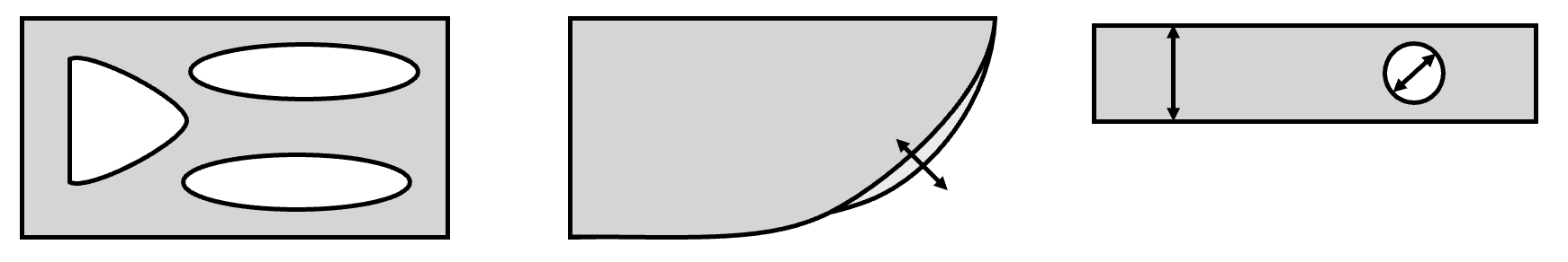
The term best depends on what we define to be the objective function of our design problem. It could be the weight to obtain light structures, it could be the cost to obtain cheap structures, or it could be CO2 emissions to obtain sustainable structures. Usually the optimization is subject to some constraints, for example a certain load that has to be endured without permanent deformation. The variables that we can change to optimize the objective function are called design variables. Depending on the choice of design variables, we generally divide three types of structural optimization problems:
The design variables describe some technical parameters of a structure, e.g. wall thickness, diameters of holes, or the cross section of beams. We seek the optimal size of these parameters in the optimization task.
The design variables describe the contour or boundary of a part. We seek the optimal shape of the part boundaries in the optimization task.
The design variables describe the presence of material in a design space. We seek the optimal distribution of material within that design space.
Before we can start optimizing structures, we need to recapitulate some basic tensor math, continuum mechanics and fundamentals of optimization, though.
During this lecture we will deal with spaces, scalars, vectors, tensors, matrices and other mathematical objects. To support understanding of which objects are used in each context, we introduce some notation rules.
A scalar variable, such as a temperature, has no direction and is completely described by a single real value. Scalars are denoted as variables in regular font, for example \[a \in \mathcal{R}.{\qquad(1.1)}\]
Most objects have some sort of direction associated with them (e.g. a velocity or a force). They are defined in a vector space \(\mathcal{R}^d\), where \(d\) is the dimension of the vector space. A vector is an element of the vector space that fulfills so-called vector axioms and is denoted in bold font, e.g. \[\textbf{a} \in \mathcal{R}^d.{\qquad(1.2)}\] In order to describe components of a vector, it is convenient to define a basis. A basis is given by a subset of vectors \(\{\mathbf{e}_1,\mathbf{e}_2,...,\mathbf{e}_d\}\) that are linearly independent and span the entire vector space. More specifically, we use an orthonormal basis (ONB) that is spanned by normalized and orthogonal vectors \(\{\mathbf{e}_i\}\). The orthogonality is expressed as \[\label{eq:orthogonality} \mathbf{e}_i \cdot \mathbf{e}_j = \delta_{ij}{\qquad(1.3)}\] with the Kronecker symbol \[\delta_{ij} = \begin{cases} 1 & \text{if } i=j \\ 0 & \text{else}. \end{cases}{\qquad(1.4)}\]
Example: Standard basis in 3D Euclidean
space
The standard basis for the three-dimensional (\(d=3\)) Euclidean space is given by the set
of three vectors \[\{\mathbf{e}_1=(1,0,0),
\mathbf{e}_2=(0,1,0), \mathbf{e}_3=(0,0,1)\}.{\qquad(1.5)}\]
With a basis, we can define a vector in terms of coordinates \((a_1, a_2, ..., a_d)\) as \[\label{eq:coordinates} \mathbf{a} = \sum_i a_i \mathbf{e}_i.{\qquad(1.6)}\] It is important to note that these coordinates depend on the basis. The same vector \(\mathbf{a}\) may be expressed with coordinates \((a_1, a_2, ..., a_d)\) for a basis \(\{\mathbf{e}_i\}\) and \((\tilde{a}_1, \tilde{a}_2, ..., \tilde{a}_d)\) for a basis \(\{\tilde{\mathbf{e}}_i\}\).
We define the inner product or scalar product of two vectors \(\mathbf{a}, \mathbf{b} \in \mathcal{R}^d\) as \[\mathbf{a} \cdot \mathbf{b} = \sum_i a_i \mathbf{e}_i \cdot \sum_j b_j \mathbf{e}_j = \sum_{i,j} a_i b_j \overbracket{(\mathbf{e}_i \cdot \mathbf{e}_j)}^{\delta_{ij}} = \sum_{i,j} a_i b_j \delta_{ij} = \sum_{i} a_i b_i{\qquad(1.7)}\] using Equation 1.3.
There are a couple of remarks at this point:
The result of the scalar product between two vectors is a scalar.
The Kronecker symbol can be interpreted as an operator that replaces an index.
A single dot always indicates a single contraction of the inner dimensions.
Some authors identify vectors with column vectors and write the dot product as a matrix product \(\mathbf{a}^\top \mathbf{b}\), where \(\mathbf{a}^\top\) denotes the transpose of \(\mathbf{a}\).
Vectors are not sufficient to describe all directional objects needed in this lecture. A stress, for example, results in a traction vector that also depends on the cutting plane defined by its normal direction. In a sense, the stress tensor combines two directions and we learn in basic mechanics courses that one index is attributed to the direction and one to the plane. We can also think about the stress tensor as a mapping from one vector to another vector or as a multi-dimensional array containing the values of \(\sigma_{ij}\).
Such tensor objects can be constructed by the outer product, tensor product, or dyadic product of two vectors \(\mathbf{a}, \mathbf{b} \in \mathcal{R}^d\) as \[\label{eq:tensorproduct} \mathbf{a} \otimes \mathbf{b} = \sum_{i,j} a_i b_j \mathbf{e}_i \otimes \mathbf{e}_j,{\qquad(1.8)}\] where the term \(\mathbf{e}_i \otimes \mathbf{e}_j\) may be interpreted as a new basis for the tensor. We may also specify such a tensor \(\mathbf{A} \in \mathcal{R}^{d \times d}\) directly as \[\mathbf{A} = \sum_{i,j} A_{ij} \mathbf{e}_i \otimes \mathbf{e}_j ,{\qquad(1.9)}\] where bold variables are used for such tensors. The entries of these tensors may be interpreted as two-dimensional arrays \[\mathbf{a} \otimes \mathbf{b} = \begin{pmatrix} a_1 b_1 & a_1 b_2 & \dots & a_1 b_d \\ a_2 b_1 & a_2 b_2 & \dots & a_2 b_d \\ \dots & \dots & \dots & \dots \\ a_d b_1 & a_d b_2 & \dots & a_d b_d \\ \end{pmatrix}_{\{\mathbf{e}_i\}}{\qquad(1.10)}\] and \[\mathbf{A} = \begin{pmatrix} A_{11} & A_{12} & \dots & A_{1d} \\ A_{21} & A_{22} & \dots & A_{2d} \\ \dots & \dots & \dots & \dots \\ A_{d1} & A_{d2} & \dots & A_{dd} \\ \end{pmatrix}_{\{\mathbf{e}_i\}}{\qquad(1.11)}\] for this specific ONB.
In fact, we can interpret some objects of the previous chapter as tensors. A vector is a first-order tensor and the Kronecker symbol can be used to define a second-order unit tensor \[\pmb{I} = \sum_{i,j} \delta_{ij} \mathbf{e}_i \otimes \mathbf{e}_j = \begin{pmatrix} 1 & 0 & \dots & 0 \\ 0 & 1 & \dots & 0 \\ \dots & \dots & \dots & \dots \\ 0 & 0 & \dots & 1 \\ \end{pmatrix}_{\{\mathbf{e}_i\}}.{\qquad(1.12)}\]
In addition, we define the trace, transpose, and inverse of a second-order tensor \(\mathbf{A} \in \mathcal{R}^{d \times d}\) as \[\begin{aligned} \textrm{tr}(\mathbf{A}) &= \sum_{i} A_{ii}, {\qquad(1.13)}\\ \mathbf{A}^\top &= \sum_{i,j} A_{ji} \mathbf{e}_i \otimes \mathbf{e}_j, \textrm{and}{\qquad(1.14)}\\ \pmb{I} &= \mathbf{A} \cdot \mathbf{A}^{-1} , {\qquad(1.15)}\end{aligned}\] respectively.
We define the tensor contraction of two second-order tensors \(\mathbf{A},\mathbf{B} \in \mathcal{R}^{d \times d}\): \[\begin{aligned} \mathbf{A} \cdot \mathbf{B} &= \sum_{i,j} A_{ij} \mathbf{e}_i \otimes \mathbf{e}_j \cdot \sum_{k,l}B_{kl} \mathbf{e}_k \otimes \mathbf{e}_l {\qquad(1.16)}\\ &= \sum_{i,j,k,l} A_{ij} B_{kl} (\mathbf{e}_i \otimes \overbracket{\mathbf{e}_j) \cdot (\mathbf{e}_k}^{\delta_{jk}} \otimes \mathbf{e}_l) {\qquad(1.17)}\\ &= \sum_{i,j,k,l} A_{ij} B_{kl} (\overbracket{\mathbf{e}_j \cdot \mathbf{e}_k}^{\delta_{jk}}) \mathbf{e}_i \otimes \mathbf{e}_l {\qquad(1.18)}\\ &= \sum_{i,j,k,l} A_{ij}B_{kl} \delta_{jk} \mathbf{e}_i \otimes \mathbf{e}_l {\qquad(1.19)}\\ &= \sum_{i,j,l} A_{ij}B_{jl} \mathbf{e}_i \otimes \mathbf{e}_l {\qquad(1.20)}\end{aligned}\] Essentially, this contracts the inner dimensions once. These are some examples of such contractions:
Example: Tensor contraction
Contraction of two first order tensors \(\mathbf{a},\mathbf{b} \in \mathcal{R}^d\):
\[\mathbf{a} \cdot \mathbf{b} = \sum_i a_i
b_i \quad \in \mathcal{R}{\qquad(1.21)}\] Contraction of two
second-order tensors \(\mathbf{A},\mathbf{B}
\in \mathcal{R}^{d \times d}\): \[\mathbf{A} \cdot \mathbf{B} = \sum_{i,j,k} A_{ij}
B_{jk} \mathbf{e}_i \otimes \mathbf{e}_k \quad \in \mathcal{R}^{d \times
d}{\qquad(1.22)}\] Contraction of a second-order tensor \(\mathbf{A} \in \mathcal{R}^{d \times d}\)
and a first-order tensor \(\mathbf{b} \in
\mathcal{R}^d\): \[\mathbf{A} \cdot
\mathbf{b} = \sum_{i,j} A_{ij} b_j \mathbf{e}_i \quad \in
\mathcal{R}^d{\qquad(1.23)}\]
We may extend the concept of outer products further to higher orders. A stiffness tensor, for example, maps a second-order strain tensor to a second-order stress tensor and thus it is a fourth-order tensor, which we denote with double-stroke capital letters. More general, a fourth order tensor may be obtained by an outer product of two second-order tensors \(\mathbf{A},\mathbf{B}\in \mathcal{R}^{d \times d}\) as \[\mathbb{C} = \mathbf{A} \otimes \mathbf{B} = \sum_{i,j,k,l} A_{ij}B_{kl} \mathbf{e}_i \otimes \mathbf{e}_j \otimes \mathbf{e}_k \otimes \mathbf{e}_l.{\qquad(1.24)}\]
We can apply the inner product multiple times. For example, we can define the double contraction of two second-order tensors \(\mathbf{A},\mathbf{B} \in \mathcal{R}^{d \times d}\): \[\begin{aligned} \mathbf{A} : \mathbf{B} &= \sum_{i,j} A_{ij} \mathbf{e}_i \otimes \mathbf{e}_j : \sum_{k,l} B_{kl} \mathbf{e}_k \otimes \mathbf{e}_l {\qquad(1.25)}\\ &= \sum_{i,j,k,l} A_{ij}B_{kl} (\mathbf{e}_i \otimes \mathbf{e}_j) : (\mathbf{e}_k \otimes \mathbf{e}_l) {\qquad(1.26)}\\ &= \sum_{i,j,k,l} A_{ij}B_{kl} \delta_{ik} \delta_{jl} {\qquad(1.27)}\\ &= \sum_{i,j} A_{ij}B_{ij} {\qquad(1.28)}\end{aligned}\]
Example: Tensor double
contraction
Double contraction of two second-order tensors \(\mathbf{A},\mathbf{B} \in \mathcal{R}^{d \times
d}\): \[\mathbf{A} : \mathbf{B} =
\sum_{i,j} A_{ij} B_{ij} \quad \in \mathcal{R}{\qquad(1.29)}\]
Double contraction of two fourth-order tensors \(\mathbb{A},\mathbb{B} \in \mathcal{R}^{d \times d
\times d \times d}\): \[\mathbb{A} :
\mathbb{B} = \sum_{i,j,k,l,m,n} A_{ijkl} B_{klmn} \mathbf{e}_i \otimes
\mathbf{e}_j \otimes \mathbf{e}_m \otimes \mathbf{e}_n \quad \in
\mathcal{R}^{d \times d \times d \times d}{\qquad(1.30)}\] Double
contraction of a fourth-order tensor \(\mathbb{A} \in \mathcal{R}^{d \times d \times d
\times d}\) and a second-order tensor \(\mathbf{B} \in \mathcal{R}^{d \times d}\):
\[\mathbb{A} : \mathbf{B} = \sum_{i,j,k,l}
A_{ijkl} B_{kl} \mathbf{e}_i \otimes \mathbf{e}_j \quad \in
\mathcal{R}^{d \times d}{\qquad(1.31)}\]
There are a couple of remarks at this point:
The number of dots in the product indicates how many inner dimensions we want to contract.
The components or matrix entries of the same tensor can be different in a different basis.
If vectors are identified with column vectors, the outer product ist written as a matrix product \(\mathbf{a} \otimes \mathbf{b} = \mathbf{a} \mathbf{b}^\top\).
In many physical processes, variables appear as tensor fields with a dependency on a spatial variable \(\mathbf{x} \in \mathcal{R}^d\). Some examples are given here:
Example: Tensor fields
A temperature field is a scalar field \[\theta: \mathcal{R}^d \rightarrow
\mathcal{R}.{\qquad(1.32)}\] A displacement field is a vector
field \[\mathbf{u}: \mathcal{R}^d \rightarrow
\mathcal{R}^d.{\qquad(1.33)}\] A stress field is a second-order
tensor field \[\pmb{\sigma}: \mathcal{R}^d
\rightarrow \mathcal{R}^{d \times d}.{\qquad(1.34)}\]
In most governing equations of physical processes, we need to compute differential operations on these fields. Therefore, the following sections introduce the most important differential operators for tensor fields assuming that the fields are differentiable and that we are using Cartesian coordinates.
A common notation for differential operations on tensor fields utilizes the Nabla operator \[\nabla = \sum_i \frac{\partial }{\partial x_i} \mathbf{e}_i = \begin{pmatrix} \frac{\partial}{\partial x_1} \\ \frac{\partial}{\partial x_2} \\ \dots \\ \frac{\partial}{\partial x_d} \\ \end{pmatrix}_{\{\mathbf{e}_i\}}{\qquad(1.35)}\] The Nabla operator may be interpreted as a first-order vector, which applies a derivative.
The gradient computes the partial derivative with respect to each spatial direction and represents this information as a higher-order tensor. We denote the gradient operator \(\nabla (\bullet)\). The resulting tensor is increased by one order as shown in the following examples:
Example: Gradient
Gradient of a scalar field \[\nabla \theta =
\sum_i \frac{\partial \theta}{\partial x_i} \mathbf{e}_i =
\begin{pmatrix}
\frac{\partial \theta}{\partial x_1} \\
\frac{\partial \theta}{\partial x_2} \\
\dots \\
\frac{\partial \theta}{\partial x_d} \\
\end{pmatrix}_{\{\mathbf{e}_i\}}{\qquad(1.36)}\] Gradient
of a vector field \[\nabla \mathbf{u} =
\sum_{i,j} \frac{\partial u_i}{\partial x_j} \mathbf{e}_i \otimes
\mathbf{e}_j
=
\begin{pmatrix}
\frac{\partial u_1}{\partial x_1} & \frac{\partial
u_1}{\partial x_2} & \dots & \frac{\partial u_1}{\partial x_d}\\
\frac{\partial u_2}{\partial x_1} & \frac{\partial
u_2}{\partial x_2} & \dots & \frac{\partial u_2}{\partial x_d}\\
\dots & \dots & \dots & \dots\\
\frac{\partial u_d}{\partial x_1} & \frac{\partial
u_d}{\partial x_2} & \dots & \frac{\partial u_d}{\partial x_d}\\
\end{pmatrix}_{\{\mathbf{e}_i\}}{\qquad(1.37)}\]
The gradient may be interpreted as a measure for how much a tensor changes in each direction.
We may compute the gradient of a gradient of a scalar field. If all the partial derivatives exits, we call the entries a Hessian.
Example: Hessian
Hessian of a scalar field \[\nabla^2 \theta =
\sum_{i,j} \frac{\partial^2 \theta}{\partial x_i \partial x_j}
\mathbf{e}_i \otimes \mathbf{e}_j
=
\begin{pmatrix}
\frac{\partial^2 \theta}{\partial x_1 \partial x_1} &
\frac{\partial^2 \theta}{\partial x_1 \partial x_2} & \dots &
\frac{\partial^2 \theta}{\partial x_1 \partial x_d}\\
\frac{\partial^2 \theta}{\partial x_2 \partial x_1} &
\frac{\partial^2 \theta}{\partial x_2 \partial x_2} & \dots &
\frac{\partial^2 \theta}{\partial x_2 \partial x_d}\\
\dots & \dots & \dots & \dots\\
\frac{\partial^2 \theta}{\partial x_d \partial x_1} &
\frac{\partial^2 \theta}{\partial x_d \partial x_2} & \dots &
\frac{\partial^2 \theta}{\partial x_d \partial x_d}\\
\end{pmatrix}_{\{\mathbf{e}_i\}}{\qquad(1.38)}\]
The divergence computes the partial derivative with respect to each spatial direction, sums these values up and represents this information as a lower-order tensor. We denote the divergence operator \(\nabla \cdot (\bullet)\). The resulting tensor is decreased by one order as shown in the following examples:
Example: Divergence
Divergence of a vector field \[\nabla \cdot
\mathbf{u} = \sum_i \frac{\partial u_i}{\partial x_i}
=
\frac{\partial u_1}{\partial x_1} + \frac{\partial u_2}{\partial
x_2} + \dots + \frac{\partial u_d}{\partial x_d}{\qquad(1.39)}\]
Divergence of a second-order tensor field \[\nabla \cdot \pmb{\sigma} = \sum_{i,j}
\frac{\partial \sigma_{ij}}{\partial x_j} \mathbf{e}_i
=
\begin{pmatrix}
\frac{\partial \sigma_{11}}{\partial x_1} + \frac{\partial
\sigma_{12}}{\partial x_2} + \frac{\partial \sigma_{13}}{\partial x_3}
\\
\frac{\partial \sigma_{21}}{\partial x_1} + \frac{\partial
\sigma_{22}}{\partial x_2} + \frac{\partial \sigma_{23}}{\partial x_3}\\
\frac{\partial \sigma_{31}}{\partial x_1} + \frac{\partial
\sigma_{32}}{\partial x_2} + \frac{\partial \sigma_{33}}{\partial x_3}
\end{pmatrix}_{\{\mathbf{e}_i\}}{\qquad(1.40)}\]
The divergence may be interpreted as the tensor field’s source. If the divergence is positive, this is a source and if it is negative, it will act as a sink.