Exercise 09 - Topology optimization for continua
Task 1 - Book shelf
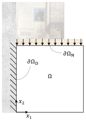
Let us consider a bookshelf that needs a support structure. The design domain is given by a unit square $x \in [0, 1]^2$ and a thickness $d=0.1$. The left boundary of the domain $\partial \Omega_D$ is fixed to the wall and the top boundary $\partial \Omega_N$ is loaded with a uniform line load representing the weight of books.
import matplotlib.pyplot as plt
import torch
from torchfem import Planar
from torchfem.materials import IsotropicElasticityPlaneStress
from torchfem.mesh import rect_quad
from tqdm import tqdm

torch.set_default_dtype(torch.double)
# Create nodes and elements for a rectangular mesh
N = 30
L = 1.0
nodes, elements = rect_quad(Nx=N + 1, Ny=N + 1, Lx=L, Ly=L)

# Define Material
material = IsotropicElasticityPlaneStress(E=1000.0, nu=0.3)

# Create model
square = Planar(nodes, elements, material)

# Define masks for boundary conditions
top = nodes[:, 1] == L
left = nodes[:, 0] == 0.0
right = nodes[:, 0] == L
tip = top & right

# Load at top
square.forces[top, 1] = -1.0 / N
square.forces[tip, 1] = -0.5 / N

# Constrained displacement at left end
square.constraints[left, :] = True

# Thickness
d = 0.1
square.thickness[:] = d
# Solve the system
u, f, sigma, F, state = square.solve()

# Compute von Mises stress
mises = torch.sqrt(
    sigma[:, 0, 0] ** 2
    - sigma[:, 0, 0] * sigma[:, 1, 1]
    + sigma[:, 1, 1] ** 2
    + 3 * sigma[:, 1, 0] ** 2
)

# Plot the result
square.plot(
    u=u,
    element_property=mises,
    cmap="viridis",
    title="von Mises stress",
    colorbar=True,
)

In addition, you are provided with a function that performs root finding with the bisection method and the computation of element surface areas from previous exercises.
def bisection(f, a, b, max_iter=50, tol=1e-12):
    # Bisection method always finds a root, if the bracket [a, b] contains a
    # sign change.
    if f(a) * f(b) > 0:
        raise Exception("No sign change in [a, b] - choose a different bracket.")
    i = 0
    while (b - a) > tol:
        c = (a + b) / 2.0
        if i > max_iter:
            raise Exception(f"Bisection did not converge in {max_iter} iterations.")
        if f(a) * f(c) > 0:
            a = c
        else:
            b = c
        i += 1
    return c
def compute_areas(model):
    areas = torch.zeros((model.n_elem))
    nodes = model.nodes[model.elements, :]
    for w, q in zip(model.etype.iweights, model.etype.ipoints):
        J = model.etype.B(q) @ nodes
        detJ = torch.linalg.det(J)
        areas[:] += w * detJ
    return areas
To save material, the bookshelf should use only 40% of the given design space, while being as stiff as possible to support many books without bending. We want to achieve this by topology optimization of the component.
To do so, we implement a topology optimization algorithm with the optimality criteria method in a function named optimize(fem, rho_0, rho_min, rho_max, V_0, iter=100, alpha=0.5, m=0.2, p=1.0, r=0.0) that takes the FEM model fem, the initial density distribution rho_0, the lower and upper density bounds rho_min, rho_max, the volume constraint V_0, the maximum iteration count iter with a default value of 100, the stabilization exponent alpha of the update rule with a default value of 0.5, the move limit m with a default value of 0.2, a SIMP penalty factor p with default 1, and a radius for sensitivity filtering r with a default 0.0. The function should return the histories of design variables and compliance values.
Recap from the lecture: The optimality criteria method updates each design variable with the rule
$$\hat{\rho}_j^{k+1} = \left(G_j^k\right)^\alpha \rho_j^k \quad \textrm{with} \quad G_j^k = \frac{-\frac{\partial C}{\partial \rho_j}(\pmb{\rho}^k)}{\mu V_j}$$
and clamps the result between the move limits
$$\rho_j^{k+1} = \textrm{clamp}\left(\hat{\rho}_j^{k+1},\; \max\left(\rho_j^-, (1-m)\rho_j^k\right),\; \min\left(\rho_j^+, (1+m)\rho_j^k\right)\right).$$
The Lagrange multiplier $\mu$ is determined with the bisection method such that the updated design satisfies the volume constraint
$$g(\mu) = \pmb{\rho}^{k+1}(\mu) \cdot \mathbf{V} - V_0 = 0.$$
The sensitivity of the compliance with the SIMP penalty $p$ is
$$\frac{\partial C}{\partial \rho_j} = -2p\rho_j^{p-1} d_j w_j(\pmb{\rho}) \quad \textrm{with the strain energy} \quad w_j = \frac{1}{2} \mathbf{u}_j \cdot \mathbf{k}^0_j \cdot \mathbf{u}_j$$
and may be smoothed with the sensitivity filter
$$\widetilde{\frac{\partial C}{\partial \rho_j}} = \frac{A_j}{\rho_j} \frac{\sum_i H_{ji} \frac{\rho_i}{A_i} \frac{\partial C}{\partial \rho_i}}{\sum_i H_{ji}} \quad \textrm{with the filter weights} \quad H_{ji} = \max\left(0, r - \textrm{dist}(i,j)\right).$$
a) Check if there is a feasible solution, i.e. if the design with minimum density has a volume smaller than the volume constraint. If not, raise an exception. Hint: You can compute the volume as the inner product of rho_min and the element volumes vols.
b) The filter weights can be precomputed before the optimization loop. Implement the computation of the filter weights if the radius is greater than 0.
Hints: Start by computing the center of each element and store it in a tensor of shape (Mx2) for M elements. Then, compute the distance between each element center using the function torch.cdist() and store it in a tensor of shape (MxM). Finally, compute the filter weights $H_{ji} = \max(0, r - \textrm{dist}(i,j))$. You can verify your result: H should be symmetric with the value $r$ on its diagonal, and plotting one of its rows with square.plot(element_property=H[465]) should show a small patch around element 465 in the center of the domain.
c) Add code that modifies the thickness according to the current design variables, solves the FEM problem, and records the compliance $C = \mathbf{f} \cdot \mathbf{u}$ in each iteration.
Hints: The element stiffness scales linearly with the thickness. Hence, you can implement the SIMP interpolation by overwriting fem.thickness with $d \rho_j^p$.
d) Compute the sensitivity of the compliance with respect to the design variables using the equation from the recap above. Hints: Computing the strain energies $w_j$ is analogous to Exercise 08 - you can extract the element-wise displacements with u[fem.elements, :].reshape(fem.n_elem, -1). The tensor k0 defined at the top of the function contains the element stiffness matrices for unit thickness $\mathbf{k}^0_j$.
e) Filter the sensitivities with the filter weights according to the equation in the recap, if the radius is greater than 0. Hint: The element volumes vols are proportional to the element areas $A_j$, hence you may use them interchangeably in the filter equation.
f) Define a function make_step(mu) that computes the design variable update for a given Lagrange parameter mu. Hints: Evaluate $G_j$ and the update rule from the recap and clamp the result between the move limits using torch.clamp().
g) Define a function g(mu) that evaluates the volume constraint. Hints: Use the make_step function to compute the design variable update and return the volume constraint violation $g(\mu)$.
h) Use the bisection method to find the Lagrange parameter that satisfies the volume constraint and append the updated design to rho. Hints: $g(\mu)$ is monotonically decreasing - a larger $\mu$ penalizes volume more and leads to smaller densities. Hence, you need a bracket $[a, b]$ with $g(a) > 0 > g(b)$. The bracket $[10^{-10}, 100]$ works for this problem.
def optimize(
    fem, rho_0, rho_min, rho_max, V_0, iter=100, alpha=0.5, m=0.2, p=1.0, r=0.0
):
    # Element stiffness matrices for unit thickness. fem.k0() includes the
    # current thickness, so we divide it out. This also keeps the function
    # correct, if it is called again on a model with modified thickness.
    k0 = torch.einsum("i,ijk->ijk", 1.0 / fem.thickness, fem.k0())

    # Histories of design variables and compliance values
    rho = [rho_0]
    C = []

    # Element volumes at full density (rho=1) with the notebook-global
    # thickness d
    vols = d * compute_areas(fem)

    # a) Check if there is a feasible solution before starting iteration
    if torch.inner(rho_min, vols) > V_0:
        raise Exception("rho_min is not compatible with V_0.")

    # b) Precompute filter weights
    if r > 0.0:
        ecenters = fem.nodes[fem.elements].mean(dim=1)
        dist = torch.cdist(ecenters, ecenters)
        H = r - dist
        H[dist > r] = 0.0

    # Iterate solutions
    for k in tqdm(range(iter), delay=0.1):
        # c) Adjust thickness, compute FEM solution, and record compliance
        fem.thickness = d * rho[k] ** p
        u, f, _, _, _ = fem.solve()
        C.append(torch.inner(f.ravel(), u.ravel()).item())

        # d) Compute sensitivities
        u_j = u[fem.elements, :].reshape(fem.n_elem, -1)
        w_j = 0.5 * torch.einsum("...i,...ij,...j", u_j, k0, u_j)
        sens = -2.0 * p * d * rho[k] ** (p - 1) * w_j

        # e) Filter sensitivities (if r provided)
        if r > 0.0:
            sens = (vols / rho[k]) * (H @ (rho[k] * sens / vols) / H.sum(dim=0))

        # f) For a certain value of mu, apply the iteration scheme
        def make_step(mu):
            G_k = -sens / (mu * vols)
            lower = torch.max(rho_min, (1 - m) * rho[k])
            upper = torch.min(rho_max, (1 + m) * rho[k])
            return torch.clamp(G_k**alpha * rho[k], lower, upper)

        # g) Constraint function
        def g(mu):
            return torch.dot(make_step(mu), vols) - V_0

        # h) Find the root of g(mu) and append the updated design to rho
        mu = bisection(g, 1e-10, 100.0)
        rho.append(make_step(mu))

    return rho, C
Once you have implemented a), you can verify it with the following checkpoint: the call below requests a volume constraint that is infeasible even at the minimum density, so your function must raise an exception.
ones = torch.ones(square.n_elem)
try:
    optimize(square, 0.9 * ones, 0.9 * ones, ones, V_0=0.05)
    print("FAILED: No exception was raised - check your feasibility test in a).")
except Exception as e:
    print(f"PASSED: Raised an exception: '{e}'")
PASSED: Raised an exception: 'rho_min is not compatible with V_0.'
i) Set up the initial design variables to $\rho_0=0.4, \rho_{min}=0.01, \rho_{max}=1.0$ for all elements and a volume constraint $V_0= 0.4 V_{max}$ with the maximum design volume $V_{max}$. The uniform design $\rho_0=0.4$ satisfies the volume constraint exactly - starting from a feasible design guarantees that a suitable Lagrange parameter exists in every iteration.
# Initial density, minimum density, maximum density
rho_0 = 0.4 * torch.ones(len(square.elements))
rho_min = 0.01 * torch.ones_like(rho_0)
rho_max = 1.0 * torch.ones_like(rho_0)

# Volume constraint (40% of maximum design volume)
vols = d * compute_areas(square)
V0 = 0.4 * vols.sum()
j) Perform the optimization with 50 iterations and the following parameters:
$$
p=3
$$
$$
r=0
$$
Self-check: Every iterate must satisfy the volume constraint exactly, i.e. torch.dot(rho_opt[-1], vols) / V0 should evaluate to 1. The compliance of the final design should be $C \approx 0.0505$.
# Optimize and visualize results
rho_opt, C_opt = optimize(square, rho_0, rho_min, rho_max, V0, iter=50, p=3.0, r=0.0)
square.plot(element_property=rho_opt[-1], cmap="gray_r")

# Self-check: volume constraint and final compliance
print(f"Volume fraction of V0: {torch.dot(rho_opt[-1], vols) / V0:.6f}")
print(f"Final compliance: {C_opt[-1]:.4f}")
100%|██████████| 50/50 [00:00<00:00, 57.82it/s]
Volume fraction of V0: 1.000000
Final compliance: 0.0505

k) Plot the evolution of the design variables and the compliance vs. iterations. To which values do the design variables converge and which parameter of the algorithm drives them there? How does the compliance evolve?
fig, ax = plt.subplots(1, 2, figsize=(10, 4))
ax[0].plot(torch.stack(rho_opt))
ax[0].set_xlabel("Iteration")
ax[0].set_ylabel(r"Values $\rho_j$")
ax[0].grid()
ax[1].plot(C_opt)
ax[1].set_xlabel("Iteration")
ax[1].set_ylabel("Compliance $C$")
ax[1].grid()
plt.tight_layout()

The left graph shows that almost all design variables converge to either the lower bound $\rho_{min}=0.01$ or the upper bound $\rho_{max}=1$: the SIMP penalty $p=3$ makes intermediate densities structurally inefficient, hence the design is driven towards a black-and-white layout. The right graph shows that the compliance decreases monotonically and settles at a constant value, indicating that the algorithm has converged.
l) Perform the optimization with 100 iterations and the following parameters $$ p=3 $$ $$ r=0.05 $$
# Optimize and visualize results
rho_opt, C_opt = optimize(square, rho_0, rho_min, rho_max, V0, iter=100, p=3.0, r=0.05)
square.plot(element_property=rho_opt[-1], cmap="gray_r")
100%|██████████| 100/100 [00:01<00:00, 54.91it/s]

m) Compare the designs from j) and l). Which numerical artifact do you observe in the unfiltered design, why does it occur, and how does the sensitivity filter suppress it?
The unfiltered design exhibits checkerboard patterns of alternating solid and void elements. These are numerical artifacts: linear shape functions overestimate the stiffness of checkerboard configurations, so the optimizer exploits them. The sensitivity filter averages the sensitivities over a neighborhood with radius $r$, which prevents members smaller than the filter radius and thereby suppresses the checkerboards.
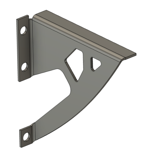
n) How do you interpret the design? Decide which manufacturing process you would like to use and use a CAD software to create a design based on your optimization.
If we want to make the bookshelf from sheet metal, this could be an interpretation:
Bonus task (optional): Repeat the optimization on a finer mesh (e.g. $N=60$) with $r=0$ and $r=0.05$. What do you observe regarding the mesh dependence of the two solutions?
# Finer mesh with the same boundary conditions
N_fine = 60
nodes_f, elements_f = rect_quad(Nx=N_fine + 1, Ny=N_fine + 1, Lx=L, Ly=L)
square_fine = Planar(nodes_f, elements_f, material)
top_f = nodes_f[:, 1] == L
tip_f = top_f & (nodes_f[:, 0] == L)
square_fine.forces[top_f, 1] = -1.0 / N_fine
square_fine.forces[tip_f, 1] = -0.5 / N_fine
square_fine.constraints[nodes_f[:, 0] == 0.0, :] = True
square_fine.thickness[:] = d

# Initial density, bounds, and volume constraint
rho_0_f = 0.4 * torch.ones(len(square_fine.elements))
rho_min_f = 0.01 * torch.ones_like(rho_0_f)
rho_max_f = 1.0 * torch.ones_like(rho_0_f)
V0_f = 0.4 * (d * compute_areas(square_fine)).sum()

# Optimize without and with filtering
rho_fine, _ = optimize(
    square_fine, rho_0_f, rho_min_f, rho_max_f, V0_f, iter=50, p=3.0, r=0.0
)
square_fine.plot(element_property=rho_fine[-1], cmap="gray_r")
rho_fine, _ = optimize(
    square_fine, rho_0_f, rho_min_f, rho_max_f, V0_f, iter=100, p=3.0, r=0.05
)
square_fine.plot(element_property=rho_fine[-1], cmap="gray_r")
100%|██████████| 50/50 [00:03<00:00, 13.49it/s]
100%|██████████| 100/100 [00:07<00:00, 12.87it/s]


Without filtering, the finer mesh converges to a considerably different design with pronounced checkerboard patches - the solution is mesh-dependent. With the same physical filter radius $r=0.05$, the optimization converges to essentially the same design as on the coarse mesh: the filter regularizes the problem and renders the solution mesh-independent.