Exercise 06 - Shape optimization of trusses

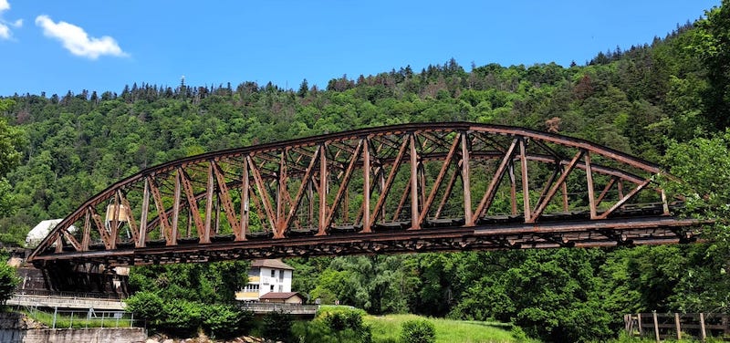
Shape optimization means that given a fixed topology of a truss, we want optimize its stiffness by modifying some node positions. In this particular example, we investigate the optimal shape of a railway bridge like in the photograph here:

from math import sqrt

import matplotlib.pyplot as plt
import torch
from torchfem import Truss

torch.set_default_dtype(torch.double)

So let's start by defining the base truss topology of the bridge without considering the exact shape for now. We create a simple rectangular bridge that has all the bars seen in the photo. The truss is fixed at the bottom left side and simply supported at the bottom right side. The load is distributed along the bottom edge of the bridge, which represents the train track.

# Dimensions
A = 17
B = 2

# Nodes
n1 = torch.linspace(0.0, 5.0, A)
n2 = torch.linspace(0.0, 0.5, B)
n1, n2 = torch.stack(torch.meshgrid(n1, n2, indexing="xy"))
nodes = torch.stack([n1.ravel(), n2.ravel()], dim=1)

# Elements
connections = []
for i in range(A - 1):
    for j in range(B):
        connections.append([i + j * A, i + 1 + j * A])
for i in range(A):
    for j in range(B - 1):
        connections.append([i + j * A, i + A + j * A])
for i in range(A - 1):
    for j in range(B - 1):
        if i >= (A - 1) / 2:
            connections.append([i + j * A, i + 1 + A + j * A])
        else:
            connections.append([i + 1 + j * A, i + A + j * A])
elements = torch.tensor(connections)

# Create Truss
bridge = Truss(nodes.clone(), elements)

# Forces at bottom edge
bridge.forces[1 : A - 1, 1] = -0.1

# Constraints by the supports
bridge.constraints[0, 0] = True
bridge.constraints[0, 1] = True
bridge.constraints[A - 1, 1] = True

# Areas
bridge.areas[:] = 1.0
bridge.moduli[:] = 500.0

# Plot
bridge.plot()

We introduce some helper functions from the last exercises. These are just copies of functions you are already familiar with.

def compute_lengths(truss):
    start_nodes = truss.nodes[truss.elements[:, 0]]
    end_nodes = truss.nodes[truss.elements[:, 1]]
    dx = end_nodes - start_nodes
    return torch.linalg.norm(dx, dim=-1)


def box_constrained_decent(
    func, x_init, x_lower, x_upper, eta=0.01, max_iter=100, tol=1e-10
):
    x = x_init.clone().requires_grad_()
    for _ in range(max_iter):
        x_old = x.clone()
        grad = torch.autograd.grad(func(x).sum(), x)[0]
        x = x - eta * grad
        x = torch.clamp(x, x_lower, x_upper)
        if torch.norm(x - x_old) < tol:
            return x
    return x


def MMA(func, x_k, L_k, U_k):
    x_lin = x_k.clone().requires_grad_()
    grads = torch.autograd.grad(func(x_lin), x_lin)[0]
    pg = grads >= 0.0
    ng = grads < 0.0
    f_k = func(x_k)

    def approximation(x):
        p = torch.zeros_like(grads)
        p[pg] = (U_k[pg] - x_k[pg]) ** 2 * grads[pg]
        q = torch.zeros_like(grads)
        q[ng] = -((x_k[ng] - L_k[ng]) ** 2) * grads[ng]
        return (
            f_k
            - torch.sum(p / (U_k - x_k) + q / (x_k - L_k))
            + torch.sum(p / (U_k - x) + q / (x - L_k))
        )

    return approximation, grads

Task 1 - Preparation of design variables

We want to restrict the shape optimization problem to the vertical displacement of the top nodes. Other nodes should not be modified - the train track should remain a flat line.

a) Create a boolean tensor mask of the same shape as nodes. It should be True for the vertical degrees of freedom of the top nodes and False for every other degree of freedom. Essentially it should mask out those nodal degrees of freedom which should be optimized.

Hints: Take a look at how the boolean constraints tensor is created in a cell above. Take a look at the plot of the bridge to see which node numbers are the top nodes.)

# Mask for design variables.
mask = torch.zeros_like(nodes, dtype=bool)
mask[A : 2 * A, 1] = True

b) Create initial values x_0 of the masked top node positions. Set limits to the deformation (x_min, x_max) such that nodes can move down by 0.4 and up by 0.5 units.

Hints: Use the mask tensor to extract the top node positions and use ravel()to flatten the tensor to get a vector of our design variables.

# Limits on design variables
x_0 = nodes[mask].ravel()
x_min = x_0 - 0.4
x_max = x_0 + 0.5

c) Compute the current volume of the truss V0. We will use this as a constraint in the optimization problem such that the optimized solution does not exceed this initial volume.

Hint: The current volume is the inner product of the current bar lengths and the cross-sectional areas of the bars.

# Compute current volume
l = compute_lengths(bridge)
V0 = torch.inner(bridge.areas, l)

Task 2 - Optimization

In this task, we will optimize the shape of the truss by minimizing the compliance of the bridge by adjusting the top nodes while keeping the volume constant:

$$ \min_{\mathbf{x}} \quad C(\mathbf{x}) = \mathbf{f} \cdot \mathbf{u}(\mathbf{x}) \\ \text{s.t.} \quad \mathbf{a} \cdot \mathbf{l}(\mathbf{x}) - V_0 \le 0\\ \quad \quad x \in [\mathbf{x}^{-}, \mathbf{x}^{+}] $$

a) Complete the objective function f(x).

Hint: Replace bridge.nodes[mask] with the design variables x to update the nodal positions of the top nodes. Use truss.solve() to compute the displacements and forces of the updated truss. Use ravel() to flatten the tensors and compute the compliance as the inner product of the forces and displacements.

def f(x):
    # Update nodes
    bridge.nodes[mask] = x
    # Solve truss with updated nodes
    u_k, f_k = bridge.solve()
    # Return compliance
    return torch.inner(f_k.ravel(), u_k.ravel())

b) Complete the constraint function g(x).

Hint: Replace bridge.nodes[mask] with the design variables x to update the nodal positions of the top nodes.

def g(x):
    # Update nodes
    bridge.nodes[mask] = x
    # Return constraint function
    return torch.inner(bridge.areas, compute_lengths(bridge)) - V0

c) Implement the updates of upper and lower asymptotes as in Exercise 04.

d) Implement the lower and upper move limits called x_min_k and x_max_k.

e) Compute the approximated functions f_tilde and g_tilde.

Hints: The MMA function returns the approximated functions f_tilde as well as the gradients of the original functions. You can assign them as follows: f_tilde, f_Grad = MMA(...).

f) Implement the approximated Lagrangian $L = \tilde{f}(\mathbf{x}) + \mu \tilde{g}(\mathbf{x}) $

g) Implement the analytical solution of x_star(mu).

Hints: This is similar to the analytical solutions in Exercise 04. Start by defining an empty stationary point x_hat filled with zeros of the same shape as f_grad. Then, define the conditions for the four cases of the analytical solution and fill the x_hat tensor accordingly by setting x_hat[cond1] = solution1 etc. Finally, clamp the results with the move limits.

h) Implement the negative dual function $-\underbar{L}(\mu) = -L(x^*(\mu), \mu)$

i) Solve for the maximum of the dual function with box_constrained_decent(...).

j) Append the solution to the list of solutions x = [$\mathbf{x}^0, \mathbf{x}^1, \mathbf{x}^2, ...$] containing the iteration steps of the optimization procedure.

s = 0.7

# Set up lists for L, U, x
L = []
U = []
x = [x_0]

# Define the initial value, lower bound, and upper bound of "mu"
mu_0 = torch.tensor([0.01])
mu_lower = torch.tensor([1e-10])
mu_upper = None

for k in range(50):
    # Update asymptotes with heuristic procedure (see Exercise 04)
    if k <= 1:
        L.append(x[k] - s * (x_max - x_min))
        U.append(x[k] + s * (x_max - x_min))
    else:
        L_k = torch.zeros_like(L[k - 1])
        U_k = torch.zeros_like(U[k - 1])
        # Shrink all oscillating asymptotes
        osci = (x[k] - x[k - 1]) * (x[k - 1] - x[k - 2]) < 0.0
        L_k[osci] = x[k][osci] - s * (x[k - 1][osci] - L[k - 1][osci])
        U_k[osci] = x[k][osci] + s * (U[k - 1][osci] - x[k - 1][osci])
        # Expand all non-oscillating asymptotes
        L_k[~osci] = x[k][~osci] - 1 / sqrt(s) * (x[k - 1][~osci] - L[k - 1][~osci])
        U_k[~osci] = x[k][~osci] + 1 / sqrt(s) * (U[k - 1][~osci] - x[k - 1][~osci])
        L.append(L_k)
        U.append(U_k)

    # Compute lower and upper move limit in this step
    x_min_k = torch.max(x_min, 0.9 * L[k] + 0.1 * x[k])
    x_max_k = torch.min(x_max, 0.9 * U[k] + 0.1 * x[k])

    # Compute the current approximation function and save gradients
    f_tilde, f_grad = MMA(f, x[k], L[k], U[k])
    g_tilde, g_grad = MMA(g, x[k], L[k], U[k])

    # Define the Lagrangian
    def lagrangian(x, mu):
        return f_tilde(x) + mu * g_tilde(x)

    # Define x_star by minimizing the Lagrangian w. r. t. x analytically
    def x_star(mu):
        x_hat = torch.zeros_like(f_grad)
        # Case 1
        cond1 = (f_grad > 0.0) & (g_grad > 0.0)
        x_hat[cond1] = x_min[cond1]
        # Case 2
        cond2 = (f_grad < 0.0) & (g_grad < 0.0)
        x_hat[cond2] = x_max[cond2]
        # Case 3
        cond3 = (f_grad > 0.0) & (g_grad < 0.0)
        roots = torch.sqrt(
            (-mu * g_grad[cond3] * (x[k][cond3] - L[k][cond3]) ** 2)
            / (U[k][cond3] - x[k][cond3]) ** 2
            / f_grad[cond3]
        )
        x_hat[cond3] = (U[k][cond3] * roots + L[k][cond3]) / (1 + roots)
        # Case 4
        cond4 = (f_grad < 0.0) & (g_grad > 0.0)
        roots = torch.sqrt(
            (-mu * g_grad[cond4] * (U[k][cond4] - x[k][cond4]) ** 2)
            / (x[k][cond4] - L[k][cond4]) ** 2
            / f_grad[cond4]
        )
        x_hat[cond4] = (U[k][cond4] + L[k][cond4] * roots) / (1 + roots)
        return torch.clamp(x_hat, x_min_k, x_max_k)

    # Define (-1 times) the dual function
    def dual_function(mu):
        return -lagrangian(x_star(mu), mu)

    # Compute the maximum of the dual function
    mu_star = box_constrained_decent(dual_function, mu_0, mu_lower, mu_upper, eta=0.01)

    # Compute current optimal point with dual solution
    x.append(x_star(mu_star).detach())

# Plot the development of design variables
plt.plot(torch.stack(x).detach())
plt.xlabel("Iteration")
plt.ylabel("Values $x_i$")
plt.show()

# Plot the optimized bridge
bridge.plot(node_labels=False)