Exercise 05 - Size optimization of trusses

We will optimize truss structures in this exercise. There is a prepared Python class for trusses called Truss and you can import it via from torchfem import Truss. The next cells show an example of how to use the truss class.

from math import log, sqrt

import torch
from torchfem import Truss
from torchfem.materials import IsotropicElasticity1D

torch.set_default_dtype(torch.double)

The truss is initialized with:

• nodes: Coordinates of the nodes (float tensor with shape Nx2)
• elements: Pairs of node IDs that are connected (integer tensor with shape Mx2)
• material: A material model (1D Material object)

In addition, we can modify default properties of the truss:

• forces: Nodal forces acting on nodes (float tensor with shape Nx2). Defaults to 0.0.
• constraints: Defines for each degree of freedom wether it is constrained (True) or not (False) (boolean tensor with shape Nx2). Defaults to False.
• displacements: Prescribed displacements at nodes (float tensor with shape Nx2). Defaults to 0.0
• areas: Cross section areas of each element (tensor with shape Mx1). Defaults to 1.0.

We can plot the object with Truss.plot().

# Define three nodes
nodes = torch.tensor([[0.0, 0.0], [1.0, 1.0], [2.0, 0.0]])

# Define two elements connecting nodes
elements = torch.tensor([[0, 1], [1, 2]])

# Define a material
material = IsotropicElasticity1D(E=1.0)

# Create truss object
truss = Truss(nodes, elements, material)

# Define a single force downwards in x_2 direction
truss.forces[1, 1] = -0.25

# Constrain all DOFs except for the central node
truss.constraints[0, :] = True
truss.constraints[2, :] = True

# Plot undeformend truss
truss.plot()

We can solve the truss problem for deformations at each node. This is done with a function Truss.solve(). The function returns displacements at each node u, forces at each node f, the stress in each bar sigma, the deformation gradient F, and a state variable state. In this lecture, we can ignore the deformation gradient (useful for large non-linear deformations) and the state (useful for non-linear materials like plasticity).

If we pass the displacements to the Truss.plot() function via (u=u), the visualization shows the deformed configuration. If we pass stresses via Truss.plot(element_property=sigma), the visualization shows color-coded stress in each bar.

# Compute the solution of the truss problem
u, f, sigma, F, state = truss.solve()

# Plot deformend truss
truss.plot(u=u)

# Plot deformend truss with stresses
truss.plot(u=u, element_property=sigma)

Task 1 - Solving a simple truss structure

Consider the three bar truss example from a previous exercise and the lecture example shown below. The coordinate origin is located at Node 1 now.

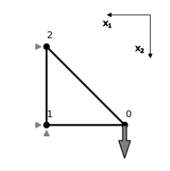
The truss is subjected to a force $P=-0.2$ indicated by the gray arrow and supports indicated by gray triangles. It has three nodes $$ \mathcal{N} = \{\mathbf{n}^0=(1,0)^\top, \mathbf{n}^1=(0,0)^\top,\mathbf{n}^2=(0,1)^\top \} $$ and three elements $$ \mathcal{E} = \{(\mathbf{n}^0, \mathbf{n}^1), (\mathbf{n}^0, \mathbf{n}^2), (\mathbf{n}^1, \mathbf{n}^2)\}. $$

Create a truss model named three_bar_truss representing this truss assuming $E=10.0$ and $A=1.0$ for each element.

a) Solve the truss problem and plot the truss in its deformed configuration with colors representing stresses in bars.

# Implement your solution here

b) Create a function named compute_lengths(truss) that accepts a truss object as input and returns a tensor containing the length of each element.

def compute_lengths(truss):
    # Implement your solution here
    pass

Task 2 - Bisection algorithm

To solve the dual problem when optimizing the truss cross sections, we will need to find the roots $\mu^*>0$ of the gradient $$ \frac{\partial \underline{\mathcal{L}}}{\partial \mu}(\mu) = \mathbf{l} \cdot \mathbf{x}^* (\mu) - V_0 = 0. $$

To prepare the search for these roots, you should implement a bisection algorithm. This algorithm performs well in this case of a highly non-linear convex optimization task, but in principle, you could also use any other gradient based algortihtm from previous exercises.

a) Write a function bisection(f, a, b, max_iter=50, tol=1e-10) that takes a function f, a bracket $[a,b]$ with $a<b$, an iteration limit max_iter and a tolerance for the solution tol. It should implement the following algorithm:

• While $b-a > tol$:
  • $c = \frac{a+b}{2}$
  • if $f(a)$ and $f(c)$ have the same sign, replace a with c
  • else replace b with c

Break the loop, if the iteration count max_iter is exceeeded to prevent infinite loops.

def bisection(f, a, b, max_iter=50, tol=1e-10):
    # Implement your solution here
    pass

b) Test the function with the function $f(x)=x^3-\log(x)-5$.

# Implement your solution here

Task 3 - Optimization algorithm

a) Implement a truss optimization algorithm according to Example 27 in the lecture. To do so, define a function optimize(truss, a_0, a_min, a_max, V_0) taking a Truss object, an initial solution of a, bounds on a a_min and a_max as well as a maximum volume V_0. You may re-use code from the previous MMA exercise.

def optimize(truss, a_0, a_min, a_max, V_0, iter=10):
    # Get stiffness matrix of truss elements
    k0 = truss.k0() / truss.areas[:, None, None]

    # Set up variables for length and s

    # Set up lists for a and L

    for k in range(iter):
        # Solve the truss problem at point a_k

        # Compute strain energy of all truss elements for the given displacement

        # Compute lower asymptotes

        # Compute lower move limit in this step

        # Define a function for the analytical solution `a_star(mu)``

        # Define a function for the analytical gradient of the dual function

        # Solve dual problem by finding the root of the gradient of the dual function
        # with the bisection algorithm

        # Compute current optimal point with dual solution

        pass

b) Test the optimization algortihm with the following code. (Works only after completing the previous tasks)

# Define initial solution and bounds
a_0 = torch.tensor([0.5, 0.2, 0.3])
a_min = 0.1 * torch.ones_like(a_0)
a_max = 1.0 * torch.ones_like(a_0)

# Define volume constraint
l = compute_lengths(three_bar_truss)
V0 = 0.5 * torch.dot(a_max, l)

# Optimize truss
a_opt = optimize(three_bar_truss, a_0, a_min, a_max, V0)

# Plot optimal solution
u, f, sigma, F, state = three_bar_truss.solve()
three_bar_truss.plot(u=u, element_property=sigma, show_thickness=True)

c) Is the optimized truss a fully stressed design?

d) Compare the solution to the analytical solution from Excercise 3. Is it the same result?

Task 4 - Your own truss

a) Create your own truss problem by defining nodes, elements, forces and constraints to your liking.

b) Solve your own truss for a prescribed distribution of cross-sectional areas. Plot the deformed truss with colored stresses.

c) Optimize the cross sections of your own truss.

d) What is the interpretation of bars having the minimum cross sectional area? What would happen if we set the minimum area to zero?