Exercise 04 - Local approximations
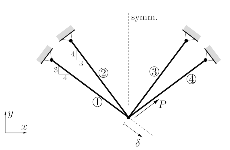
The volume of a four-bar truss should be minimized under the displacement constraint $\delta \le \delta_0$. There is a force $P>0$ acting along the direction of bar 4. All bars have identical lengths $l$ and identical Young's moduli $E$. The modifiable structural variables are the cross sectional areas $A_1=A_4$ and $A_2=A_3$. We define $A_0 = Pl / (10\delta_0E)$ and constrain the variables $0.2A_0 \le A_j \le 2.5 A_0$. Then we can use dimensionless design variables $a_j=A_j/A_0 \in [0.2, 2.5]$.
Credits: Peter W. Christensen and Anders Klarbring. An Introduction to Structural Optimization. Springer Netherlands, 2008.
from math import sqrt

import matplotlib.pyplot as plt
import torch
from torchfem.utils import plot_contours
Task 1 - Defining the constrained optimization problem
a) Compute the objective function $f(\mathbf{a})$ that should be minimized and define it as Python function that accepts inputs tensors of the shape [..., 2].
# Define f(a)
def f(a):
    pass
b) Compute the constraint function $g(\mathbf{a})$ for $\delta_0=0.1$ and define it as Python function that accepts inputs tensors of the shape [..., 2].
# Define g(a)
def g(a):
    pass
c) Summarize the optimization problem statement with all constraints.
Task 2 - CONLIN
a) Implement a function named CONLIN(func, a_k) that computes a CONLIN approximation of the function func at position a_k. CONLIN should return an approximation function that can be evaluated at any point a.
def CONLIN(func, a_k):
    # Implement your solution here
    a_lin = a_k.clone().requires_grad_()
    gradients = torch.autograd.grad(func(a_lin).sum(), a_lin)[0]

    def approximation(a):
        # Implement your solution here
        pass

    return approximation
b) Test your CONLIN approximation with the following code. Does the plot match your expectations?
def test_function(x):
    return 5.0 / x + 2.0 * x


x = torch.linspace(0, 10, 100)[:, None]
x_0 = torch.tensor([1.0])
test_approximation = CONLIN(test_function, x_0)
plt.plot(x, test_function(x), label="f(x)")
plt.plot(x, [test_approximation(x_i) for x_i in x], label=f"CONLIN at x={x_0.item()}")
plt.axvline(x_0, color="tab:orange", linestyle="--")
plt.legend()
plt.xlabel("x")
plt.ylabel("f(x)")
plt.xlim(0, 10)
plt.ylim(0, 25)
plt.show()
c) Solve the problem with sequential CONLIN approximations starting from $\mathbf{a}^0 = (2,1)^\top$ with the dual method. Record all intermediate points $\mathbf{a}^0, \mathbf{a}^1, \mathbf{a}^2, ...$ in a list called a for later plotting.
You will need to compute minima and maxima in this procedure, hence you are given the box_constrained_descent method from the previous exercise to perform these operations. The method is slightly modified:
- It takes extra arguments that can be passed to the function, e.g. by
box_constrained_descent(..., mu=1.0) - It returns only the final result and not all intermediate steps
def box_constrained_descent(
    func, x_init, x_lower, x_upper, eta=0.1, max_iter=100, **extra_args
):
    x = x_init.clone().requires_grad_()
    for _ in range(max_iter):
        grad = torch.autograd.grad(func(x, **extra_args).sum(), x)[0]
        x = x - eta * grad
        x = torch.clamp(x, x_lower, x_upper)
    return x
# Define the initial values, lower bound, and upper bound of "a"
a_0 = torch.tensor([2.0, 1.0])
a_lower = torch.tensor([0.2, 0.2])
a_upper = torch.tensor([2.5, 2.5])

# Define the initial value, lower bound, and upper bound of "mu"
mu_0 = torch.tensor([10.0])
mu_lower = torch.tensor([1e-10])
mu_upper = None

# Define list of a
a = [a_0]

# Implement your solution here
d) Test your optimization with the following code. Does the plot match your expectations?
# Plotting domain
a_1 = torch.linspace(0.1, 3.0, 200)
a_2 = torch.linspace(0.1, 3.0, 200)
a_grid = torch.stack(torch.meshgrid(a_1, a_2, indexing="xy"), dim=2)

# Make a plot
plot_contours(
    a_grid,
    f(a_grid),
    paths={"CONLIN": a},
    box=[a_lower, a_upper],
    opti=[a[-1][0], a[-1][1]],
    figsize=(5, 5),
)
plt.contour(a_1, a_2, g(a_grid), [0], colors="k", linewidths=3)
plt.contourf(a_1, a_2, g(a_grid), [0, 1], colors="gray", alpha=0.5)
plt.show()
e) This implementation is relatively slow. How could it be accelerated?
Task 3 - MMA
a) Implement a function named MMA(func, a_k, L_k, U_k) that computes a MMA approximation of the function func at position a_k with lower asymptotes L_k and upper asymptotes U_k. MMA should return an approximation function that can be evaluated at any point a.
def MMA(func, a_k, L_k, U_k):
    a_lin = a_k.clone().requires_grad_()
    grads = torch.autograd.grad(func(a_lin), a_lin)[0]

    def approximation(a):
        # Implement your solution here
        pass

    return approximation
b) Test your MMA approximation with the following code. Does the plot match your expectations?
def test_function(x):
    return 5.0 / x + 2.0 * x


x = torch.linspace(0, 10, 100)[:, None]
x_0 = torch.tensor([1.0])
L_0 = torch.tensor([0.1])
U_0 = torch.tensor([8.0])
x_test = torch.linspace(L_0.item(), U_0.item(), 100)[:, None]
test_approximation = MMA(test_function, x_0, L_0, U_0)
plt.plot(x, test_function(x), label="f(x)")
plt.plot(x_test, [test_approximation(x_i) for x_i in x_test], label=f"MMA at x={x_0}")
plt.axvline(x_0, color="tab:orange", linestyle="--")
plt.axvline(L_0, color="black", linestyle="--")
plt.axvline(U_0, color="black", linestyle="--")
plt.legend()
plt.xlabel("x")
plt.ylabel("f(x)")
plt.xlim(0, 10)
plt.ylim(-5, 25)
plt.show()
c) Solve the problem with sequential MMA approximations starting from $\mathbf{a}^0 = (2,1)^\top$ with the dual method. Record all intermediate points $\mathbf{a}^0, \mathbf{a}^1, \mathbf{a}^2, ...$ in a list called a for the asymptote updates and later plotting.
# Define the initial values, lower bound, and upper bound of "a"
a_0 = torch.tensor([2.0, 1.0])
a_lower = torch.tensor([0.2, 0.2])
a_upper = torch.tensor([2.5, 2.5])

# Define the initial value, lower bound, and upper bound of "mu"
mu_0 = torch.tensor([10.0])
mu_lower = torch.tensor([0.0])
mu_upper = torch.tensor([1000000000.0])

# Define lists for  a, L, and U
a = [a_0]

# Implement your solution here
d) Test your optimization with the following code. Does the plot match your expectations?
# Plotting domain
a_1 = torch.linspace(0.1, 3.0, 200)
a_2 = torch.linspace(0.1, 3.0, 200)
a_grid = torch.stack(torch.meshgrid(a_1, a_2, indexing="xy"), dim=2)

# Make a plot
plot_contours(
    a_grid,
    f(a_grid),
    paths={"MMA": a},
    box=[a_lower, a_upper],
    opti=[a[-1][0], a[-1][1]],
    figsize=(5, 5),
)
plt.contour(a_1, a_2, g(a_grid), [0], colors="k", linewidths=3)
plt.contourf(a_1, a_2, g(a_grid), [0, 1], colors="gray", alpha=0.5)
plt.show()
e) This implementation is relatively slow. How could it be accelerated?