Exercise 04 - Local approximations
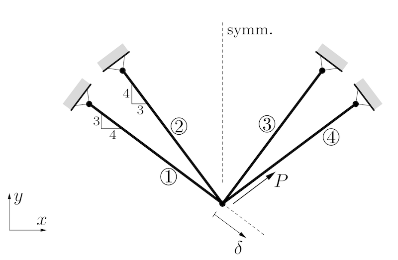
The volume of a four-bar truss should be minimized under the displacement constraint $\delta \le \delta_0$. There is a force $P>0$ acting along the direction of bar 4. All bars have identical lengths $l$ and identical Young's moduli $E$. The modifiable structural variables are the cross sectional areas $A_1=A_4$ and $A_2=A_3$. We define $A_0 = Pl / (10\delta_0E)$ and constrain the variables $0.2A_0 \le A_j \le 2.5 A_0$. Then we can use dimensionless design variables $a_j=A_j/A_0 \in [0.2, 2.5]$.
Credits: Peter W. Christensen and Anders Klarbring. An Introduction to Structural Optimization. Springer Netherlands, 2008.
from math import sqrt

import matplotlib.pyplot as plt
import torch
from torchfem.utils import plot_contours
Task 1 - Defining the constrained optimization problem
a) Compute the objective function $f(\mathbf{a})$ that should be minimized and define it as Python function that accepts inputs tensors of the shape [..., 2].
The total volume is $$ V = l A_1 + l A_2 + l A_3 + l A_4 = 2l A_1 + 2l A_2.$$ Substituting $A_j = a_j A_0$ gives $$ V = 2l A_0 (a_1 + a_2).$$ The factor in front of the brackets is a positive constant, which we can neglect for the optimization task itself. Hence, we can simplify the function to $$f(\mathbf{a}) = a_1 + a_2.$$
def f(a):
    return a[..., 0] + a[..., 1]
b) Compute the constraint function $g(\mathbf{a})$ for $\delta_0=0.1$ and define it as Python function that accepts inputs tensors of the shape [..., 2].
A free body diagram of the free node gives $$ - \frac{4}{5} P_1 - \frac{3}{5} P_2 + \frac{3}{5}P_3 + \frac{4}{5} P_4 + \frac{4}{5} P = 0 $$ $$ \frac{3}{5} P_1 + \frac{4}{5} P_2 + \frac{4}{5}P_3 + \frac{3}{5} P_4 + \frac{3}{5} P = 0 $$ In addition, the kinematics give us the following relation for the elongation of each bar $\Delta u_j$: $$ \frac{4}{5} u_1 - \frac{3}{5} u_2 = \Delta u_1$$ $$ \frac{3}{5} u_1 - \frac{4}{5} u_2 = \Delta u_2 $$ $$ -\frac{3}{5} u_1 - \frac{4}{5} u_2 = \Delta u_3 $$ $$ -\frac{4}{5} u_1 - \frac{3}{5} u_2 = \Delta u_4 $$ Substituting the displacements into the elastic relations and using $A_1=A_4$ and $A_2=A_3$ gives $$P_1 = \frac{E}{5l} A_1 (4u_1-3u_2)$$ $$P_2 = \frac{E}{5l} A_2 (3u_1-4u_2)$$ $$P_3 = \frac{E}{5l} A_2 (-3u_1-4u_2)$$ $$P_4 = \frac{E}{5l} A_1 (-4u_1-3u_2)$$ Substituting these expression into the first two equations of the free body diagram yields $$u_1(32A_1+18A_2)=20 \frac{Pl}{E}$$ $$u_2(18A_1+32A_2)=15 \frac{Pl}{E}$$ which can be solved for $$u_1 = \frac{10}{16a_1+9a_2}$$ $$u_2 = \frac{7.5}{9a_1+16a_2}$$ using the definition of $A_0$. Finally, we can compute the displacement $$\delta = \Delta u_1 = \frac{4}{5} u_1 - \frac{3}{5} u_2 = \frac{8}{16a_1+9a_2} - \frac{4.5}{9a_1+16a_2}$$ and define $$g(\mathbf{a}) = \frac{8}{16a_1+9a_2} - \frac{4.5}{9a_1+16a_2} - 0.1.$$
def g(a):
    return (
        8 / (16 * a[..., 0] + 9 * a[..., 1])
        - 4.5 / (9 * a[..., 0] + 16 * a[..., 1])
        - 0.1
    )
c) Summarize the optimization problem statement with all constraints.
$$\min_\mathbf{a} f(\mathbf{a}) = a_1 + a_2$$ $$\text{s.t.} \quad g(\mathbf{a}) = \frac{8}{16a_1+9a_2} - \frac{4.5}{9a_1+16a_2} - 0.1 \le 0$$ $$\quad a_1 \in [0.2, 2.5], a_2 \in [0.2, 2.5]$$
Task 2 - CONLIN
a) Implement a function named CONLIN(func, a_k) that computes a CONLIN approximation of the function func at position a_k. CONLIN should return an approximation function that can be evaluated at any point a.
def CONLIN(func, a_k):
    a_lin = a_k.clone().requires_grad_()
    gradients = torch.autograd.grad(func(a_lin), a_lin)[0]

    def approximation(a):
        res = func(a_k)
        for j, grad in enumerate(gradients):
            if grad < 0.0:
                Gamma = a_k[j] / a[j]
            else:
                Gamma = 1.0
            res += grad * Gamma * (a[j] - a_k[j])
        return res

    return approximation
b) Test your CONLIN approximation with the following code. Does the plot match your expectations?
def test_function(x):
    return 5.0 / x + 2.0 * x


x = torch.linspace(0, 10, 100)[:, None]
x_0 = torch.tensor([1.0])
test_approximation = CONLIN(test_function, x_0)
plt.plot(x, test_function(x), label="f(x)")
plt.plot(x, [test_approximation(x_i) for x_i in x], label=f"CONLIN at x={x_0.item()}")
plt.axvline(x_0, color="tab:orange", linestyle="--")
plt.legend()
plt.xlabel("x")
plt.ylabel("f(x)")
plt.xlim(0, 10)
plt.ylim(0, 25)
plt.show()

c) Solve the problem with sequential CONLIN approximations starting from $\mathbf{a}^0 = (2,1)^\top$ with the dual method. Record all intermediate points $\mathbf{a}^0, \mathbf{a}^1, \mathbf{a}^2, ...$ in a list called a for later plotting.
You will need to compute minima and maxima in this procedure, hence you are given the box_constrained_descent method from the previous exercise to perform these operations. The method is slightly modified:
- It takes extra arguments that can be passed to the function, e.g. by
box_constrained_descent(..., mu=1.0) - It returns only the final result and not all intermediate steps
def box_constrained_descent(
    func, x_init, x_lower, x_upper, eta=0.1, max_iter=100, **extra_args
):
    x = x_init.clone().requires_grad_()
    for _ in range(max_iter):
        grad = torch.autograd.grad(func(x, **extra_args), x)[0]
        x = x - eta * grad
        x = torch.clamp(x, x_lower, x_upper)
    return x
# Define the initial values, lower bound, and upper bound of "a"
a_0 = torch.tensor([2.0, 1.0], requires_grad=True)
a_lower = torch.tensor([0.2, 0.2])
a_upper = torch.tensor([2.5, 2.5])

# Define the initial value, lower bound, and upper bound of "mu"
mu_0 = torch.tensor([10.0])
mu_lower = torch.tensor([1e-10])
mu_upper = None

# Save intermediate values
a = [a_0]

for k in range(3):
    # Compute the current approximation function:
    g_tilde = CONLIN(g, a[k])

    # Define the Lagrangian
    def lagrangian(a, mu):
        return f(a) + mu * g_tilde(a)

    # Define a_star by minimizing the Lagrangian w. r. t. a numerically
    def a_star(mu):
        return box_constrained_descent(lagrangian, a[k], a_lower, a_upper, mu=mu)

    # Define (-1 times) the dual function
    def dual_function(mu):
        return -lagrangian(a_star(mu), mu)

    # Compute the maximum of the dual function
    mu_k = box_constrained_descent(dual_function, mu_0, mu_lower, mu_upper, eta=10.0)

    # Compute the next a_k from mu_k and append it to a
    a.append(a_star(mu_k))
d) Test your optimization with the following code. Does the plot match your expectations?
# Plotting domain
a_1 = torch.linspace(0.1, 3.0, 200)
a_2 = torch.linspace(0.1, 3.0, 200)
a_grid = torch.stack(torch.meshgrid(a_1, a_2, indexing="xy"), dim=2)

# Make a plot
plot_contours(
    a_grid,
    f(a_grid),
    paths={"CONLIN": a},
    box=[a_lower, a_upper],
    opti=[a[-1][0], a[-1][1]],
    figsize=(5, 5),
)
plt.contour(a_1, a_2, g(a_grid), [0], colors="k", linewidths=3)
plt.contourf(a_1, a_2, g(a_grid), [0, 1], colors="gray", alpha=0.5)
plt.show()

e) This implementation is relatively slow. How could it be accelerated?
We could compute gradients analytically. This is an example giving the same result, but much faster.
The approximated function is separable, i.e. we can state the following for a stationary point $$ \frac{\partial \mathcal{L}}{\partial a_j} = \begin{cases} 1 + \mu \frac{\partial g}{\partial a_j}(\mathbf{a}^k) &\quad \text{if} \frac{\partial g}{\partial a_j}(\mathbf{a}^k) \ge 0\\ 1 + \mu \frac{\partial g}{\partial a_j}(\mathbf{a}^k) \left(\frac{a_j^k}{a_j}\right)^2 &\quad \text{else} \end{cases} $$ If this should equal 0, we can solve it for the optimum $a^*_j$ as $$ a^*_j = \begin{cases} a_j^l &\quad \text{if} \frac{\partial g}{\partial a_j}(\mathbf{a}^k) \ge 0\\ \sqrt{-\mu \frac{\partial g}{\partial a_j}(\mathbf{a}^k)\left(a_j^k\right)^2} &\quad \text{else} \end{cases} $$ where we use the fact that a linear approximation with a positive slope will have its minimum at the lowest value of $a$, i.e. $a_j^l$.
# Save intermediate values
a = [a_0]

for k in range(3):
    # Compute the current approximation function:
    g_tilde = CONLIN(g, a[k])

    # Define the Lagrangian
    def lagrangian(a, mu):
        return f(a) + mu * g_tilde(a)

    # Define a_star by minimizing the Lagrangian w. r. t. a analytically
    a_lin = a[k].clone().requires_grad_()
    gradients = torch.autograd.grad(g(a_lin), a_lin)[0]

    def a_star(mu):
        a_hat = torch.zeros_like(gradients)
        pg = gradients >= 0
        ng = gradients < 0
        a_hat[pg] = a_lower[pg]
        a_hat[ng] = torch.sqrt(-mu * gradients[ng] * a[k][ng] ** 2)
        return torch.clamp(a_hat, a_lower, a_upper)

    # Define (-1 times) the dual function
    def dual_function(mu):
        return -lagrangian(a_star(mu), mu)

    # Compute the maximum of the dual function
    mu_k = box_constrained_descent(dual_function, mu_0, mu_lower, mu_upper, eta=10.0)

    # Compute the next a_k from mu_k and append it to a
    a.append(a_star(mu_k))
# Make a plot
plot_contours(
    a_grid,
    f(a_grid),
    paths={"CONLIN analytical": a},
    box=[a_lower, a_upper],
    opti=[a[-1][0], a[-1][1]],
    figsize=(5, 5),
)
plt.contour(a_1, a_2, g(a_grid), [0], colors="k", linewidths=3)
plt.contourf(a_1, a_2, g(a_grid), [0, 1], colors="gray", alpha=0.5)
plt.show()

Task 3 - MMA
a) Implement a function named MMA(func, a_k, L_k, U_k) that computes a MMA approximation of the function func at position a_k with lower asymptotes L_k and upper asymptotes U_k. MMA should return an approximation function that can be evaluated at any point a.
def MMA(func, a_k, L_k, U_k):
    a_lin = a_k.clone().requires_grad_()
    grads = torch.autograd.grad(func(a_lin), a_lin)[0]
    pg = grads >= 0
    ng = grads < 0.0

    def approximation(a):
        p = torch.zeros_like(grads)
        p[pg] = (U_k[pg] - a_k[pg]) ** 2 * grads[pg]
        q = torch.zeros_like(grads)
        q[ng] = -((a_k[ng] - L_k[ng]) ** 2) * grads[ng]
        r = func(a_k) - torch.sum(p / (U_k - a_k) + q / (a_k - L_k))
        return r + torch.sum(p / (U_k - a) + q / (a - L_k))

    return approximation
b) Test your MMA approximation with the following code. Does the plot match your expectations?
def test_function(x):
    return 5.0 / x + 2.0 * x


x = torch.linspace(0, 10, 100)[:, None]
x_0 = torch.tensor([1.0])
L_0 = torch.tensor([0.1])
U_0 = torch.tensor([8.0])
x_test = torch.linspace(L_0.item(), U_0.item(), 100)[:, None]
test_approximation = MMA(test_function, x_0, L_0, U_0)
plt.plot(x, test_function(x), label="f(x)")
plt.plot(x_test, [test_approximation(x_i) for x_i in x_test], label=f"MMA at x={x_0}")
plt.axvline(x_0, color="tab:orange", linestyle="--")
plt.axvline(L_0, color="black", linestyle="--")
plt.axvline(U_0, color="black", linestyle="--")
plt.legend()
plt.xlabel("x")
plt.ylabel("f(x)")
plt.xlim(0, 10)
plt.ylim(-5, 25)
plt.show()

c) Solve the problem with sequential MMA approximations starting from $\mathbf{a}^0 = (2,1)^\top$ with the dual method. Record all intermediate points $\mathbf{a}^0, \mathbf{a}^1, \mathbf{a}^2, ...$ in a list called a for the asymptote updates and later plotting.
# Define the initial values, lower bound, and upper bound of "a"
a_0 = torch.tensor([2.0, 1.0], requires_grad=True)
a_lower = torch.tensor([0.2, 0.2])
a_upper = torch.tensor([2.5, 2.5])

# Define the initial value, lower bound, and upper bound of "mu"
mu_0 = torch.tensor([10.0])
mu_lower = torch.tensor([1e-10])
mu_upper = None

# Save intermediate values
a = [a_0]
L = []
U = []

# Define factor s for shrinkage and growth of asymptotes
s = 0.7

for k in range(5):
    # Update asymptotes with heuristic procedure
    if k <= 1:
        L.append(a[k] - s * (a_upper - a_lower))
        U.append(a[k] + s * (a_upper - a_lower))
    else:
        L_k = torch.zeros_like(L[k - 1])
        U_k = torch.zeros_like(U[k - 1])
        # Shrink all oscillating asymptotes
        osci = (a[k] - a[k - 1]) * (a[k - 1] - a[k - 2]) < 0.0
        L_k[osci] = a[k][osci] - s * (a[k - 1][osci] - L[k - 1][osci])
        U_k[osci] = a[k][osci] + s * (U[k - 1][osci] - a[k - 1][osci])
        # Expand all non-oscillating asymptotes
        L_k[~osci] = a[k][~osci] - 1.0 / sqrt(s) * (a[k - 1][~osci] - L[k - 1][~osci])
        U_k[~osci] = a[k][~osci] + 1.0 / sqrt(s) * (U[k - 1][~osci] - a[k - 1][~osci])
        L.append(L_k)
        U.append(U_k)

    # Compute lower move limit in this step
    a_lower_k = torch.max(a_lower, 0.9 * L[k] + 0.1 * a[k])
    a_upper_k = torch.min(a_upper, 0.9 * U[k] + 0.1 * a[k])

    # Compute the current approximation function:
    g_tilde = MMA(g, a[k], L[k], U[k])

    # Define the Lagrangian
    def lagrangian(a, mu):
        return f(a) + mu * g_tilde(a)

    # Define a_star by minimizing the Lagrangian w. r. t. a
    def a_star(mu):
        return box_constrained_descent(lagrangian, a[k], a_lower_k, a_upper_k, mu=mu)

    # Define (-1 times) the dual function
    def dual_function(mu):
        return -lagrangian(a_star(mu), mu)

    # Compute the maximum of the dual function
    mu_k = box_constrained_descent(dual_function, mu_0, mu_lower, mu_upper, eta=10.0)

    # Compute the next a_k from mu_k and append it to a
    a.append(a_star(mu_k))
d) Test your optimization with the following code. Does the plot match your expectations?
# Plotting domain
a_1 = torch.linspace(0.1, 3.0, 200)
a_2 = torch.linspace(0.1, 3.0, 200)
a_grid = torch.stack(torch.meshgrid(a_1, a_2, indexing="xy"), dim=2)

# Make a plot
plot_contours(
    a_grid,
    f(a_grid),
    paths={"MMA": a},
    box=[a_lower, a_upper],
    opti=[a[-1][0], a[-1][1]],
    figsize=(5, 5),
)
plt.contour(a_1, a_2, g(a_grid), [0], colors="k", linewidths=3)
plt.contourf(a_1, a_2, g(a_grid), [0, 1], colors="gray", alpha=0.5)
plt.show()

e) This implementation is relatively slow. How could it be accelerated?
We could compute gradients analytically. This is an example giving the same result, but much faster.
The approximated function is separable, i.e. we can formulate the stationary condition as $$ \frac{\partial \mathcal{L}}{\partial a_j} = \begin{cases} 1 + \mu \left(\frac{U_j^k-a_j^k}{U_j^k-a_j}\right)^2\frac{\partial g}{\partial a_j}(\mathbf{a}^k) &\quad \text{if} \frac{\partial g}{\partial a_j}(\mathbf{a}^k) \ge 0\\ 1 + \mu \left(\frac{a_j^k-L_j^k}{a_j-L_j^k}\right)^2\frac{\partial g}{\partial a_j}(\mathbf{a}^k) &\quad \text{else} \end{cases} $$ If this should equal 0, we can solve it for $a^*_j$ as $$ a^*_j = \begin{cases} a_j^l &\quad \text{if} \frac{\partial g}{\partial a_j}(\mathbf{a}^k) \ge 0\\ L_j^k+\sqrt{-\mu(a_j^k-L_j^k)^2\frac{\partial g}{\partial a_j}(\mathbf{a}^k)} &\quad \text{else} \end{cases} $$ where we use the fact that a linear approximation with a positive slope will have its minimum at the lowest value of $a$, i.e. $a_j^l$.
# Save intermediate values
a = [a_0]
L = []
U = []

# Define factor s for shrinkage and growth of asymptotes
s = 0.7

for k in range(5):
    # Update asymptotes with heuristic procedure
    if k <= 1:
        L.append(a[k] - s * (a_upper - a_lower))
        U.append(a[k] + s * (a_upper - a_lower))
    else:
        L_k = torch.zeros_like(L[k - 1])
        U_k = torch.zeros_like(U[k - 1])
        # Shrink oscillating asymptotes
        osci = (a[k] - a[k - 1]) * (a[k - 1] - a[k - 2]) < 0.0
        L_k[osci] = a[k][osci] - s * (a[k - 1][osci] - L[k - 1][osci])
        U_k[osci] = a[k][osci] + s * (U[k - 1][osci] - a[k - 1][osci])
        # Expand non-oscillating asymptotes
        L_k[~osci] = a[k][~osci] - 1.0 / sqrt(s) * (a[k - 1][~osci] - L[k - 1][~osci])
        U_k[~osci] = a[k][~osci] + 1.0 / sqrt(s) * (U[k - 1][~osci] - a[k - 1][~osci])
        L.append(L_k)
        U.append(U_k)

    # Compute lower move limit in this step
    a_lower_k = torch.max(a_lower, 0.9 * L[k] + 0.1 * a[k])
    a_upper_k = torch.min(a_upper, 0.9 * U[k] + 0.1 * a[k])

    # Compute the current approximation function:
    g_tilde = MMA(g, a[k], L[k], U[k])

    # Define the Lagrangian
    def lagrangian(a, mu):
        return f(a) + mu * g_tilde(a)

    # Define a_star by minimizing the Lagrangian w. r. t. a analytically
    a_lin = a[k].clone().requires_grad_()
    gradients = torch.autograd.grad(g(a_lin), a_lin)[0]

    def a_star(mu):
        a_hat = torch.zeros_like(gradients)
        pg = gradients >= 0
        ng = gradients < 0
        a_hat[pg] = a_lower[pg]
        a_hat[ng] = L[k][ng] + torch.sqrt(
            -mu * (a[k][ng] - L[k][ng]) ** 2 * gradients[ng]
        )

        return torch.clamp(a_hat, a_lower_k, a_upper_k)

    # Define (-1 times) the dual function
    def dual_function(mu):
        return -lagrangian(a_star(mu), mu)

    # Compute the maximum of the dual function
    mu_k = box_constrained_descent(dual_function, mu_0, mu_lower, mu_upper, eta=10.0)

    # Compute the next a_k from mu_k and append it to a
    a.append(a_star(mu_k))
# Make a plot
plot_contours(
    a_grid,
    f(a_grid),
    paths={"MMA analytical": a},
    box=[a_lower, a_upper],
    opti=[a[-1][0], a[-1][1]],
    figsize=(5, 5),
)
plt.contour(a_1, a_2, g(a_grid), [0], colors="k", linewidths=3)
plt.contourf(a_1, a_2, g(a_grid), [0, 1], colors="gray", alpha=0.5)
plt.show()
