In the previous chapter, we drew the analogy between an optimization
problem and the search for the lowest point in a mountainous landscape.
We may continue with this analogy and make it a bit more realistic:
Previously, the hiking person was able to access any point in the
mountain range \(\mathcal{R}^d\).
However, in reality we might find a couple of constraints in that
mountainous landscape. Someone might have put fences in the landscape
and we are not able to cross these fences or we are restricted to a
hiking path and cannot leave that path.
These additional constraints make the optimization harder - the
optimum that is achievable for us might be just "at a fence" and not the
global optimum of the unrestricted function. We denote the general form
of a constrained optimization problem as \[\begin{aligned}
\min_{\mathbf{x}} \quad & f(\mathbf{x})\\
\textrm{s.t.} \quad & g_i(\mathbf{x}) \le 0 &i \in
[1, n]\\
& h_j(\mathbf{x}) = 0 &j \in [1,
m]\\
& \mathbf{x} \in \mathcal{X} \subset
\mathcal{R}^d\\
\end{aligned}
\label{eq:constrained_optimization}{\qquad(3.1)}\] with \(n\) inequality constraints \(g_i : \mathcal{X} \rightarrow \mathcal{R}\)
("fences"), \(m\) equality constraints
\(h_j: \mathcal{X} \rightarrow
\mathcal{R}\) ("hiking paths") and a box constraint \(\mathbf{x} \in \mathcal{X}\) ("allowed
zone" in the mountain range). A constrained optimization problem is
strictly convex, if the set \(\mathcal{X}\) is strictly convex, the
objective function is strictly convex and the constraints are strictly
convex.
Learning Objectives
After studying this chapter and finishing the exercise, you should be
able to
treat box constraints in gradient descent methods with projected
gradients
formulate Lagrangian functions of constrained optimization
problems
apply the Karush-Kuhn Tucker conditions to find the optimum of a
convex constrained optimization problem
explain the term Lagrangian duality and in which cases
the dual formulation is beneficial
apply the Lagrangian duality method to solve convex separable
problems
3.1 Box constraints
First, we neglect the equality constraints and inequality constraints
in the problem 3.1, i.e.
\(m=0, n=0\), and focus on box
constraints \(\mathbf{x} \in
\mathcal{X}\). Box constraint means that the variables
are limited to an upper and lower bound \(\mathbf{x}^+\) and \(\mathbf{x}^-\), respectively. For example,
design variables in structural optimization could be diameters of beams,
which cannot become negative or should not exceed a certain maximum
producible size.
These constraints are probably the most straightforward constraints
in an optimization problem and in a one-dimensional optimization problem
we can deal with them simply by clamping the scalar variable as \[x^* = \textrm{clamp}(\hat{x}, x^-, x^+) =
\min(\max(\hat{x}, x^-), x^+){\qquad(3.2)}\] with the stationary
point \(\hat{x}\), the lower bound
\(x^-\) and the upper bound \(x^+\). However, clamping the stationary
point in each dimension of a multi-dimensional problem would not result
in the optimal point, as illustrated by the green point in the next
example (Niculae
2020).
One method to deal with box constraints in multi-dimensional
optimization problems is the projected gradient method. In this method
we project each step of a gradient descent back to the domain as \[\mathbf{x}^{k+1} = P(\mathbf{x}^k -\eta \nabla
f(\mathbf{x}^k)){\qquad(3.3)}\] with a projection function \(P: \mathcal{R}^d \rightarrow \mathcal{X}\).
In case of box constraints, this projection is simply clamping the
values to \(\mathcal{X}\) by \[P(\mathbf{x}) = \textrm{clamp}(\mathbf{x},
\mathbf{x}^-, \mathbf{x}^+) = \min(\max(\mathbf{x}, \mathbf{x}^-),
\mathbf{x}^+).{\qquad(3.4)}\] Here, all operators (\(\max\), \(\min\) and \(\textrm{clamp}\)) are applied as point-wise
comparisons to the components of its inputs.
Example: Box constraints
We want to find the solution of the following quadratic optimization
problem \[\begin{aligned}
\min_{\mathbf{x}} \quad & f(\mathbf{x})=
(\mathbf{x}-\tilde{\mathbf{x}}) \cdot \mathbf{Q} \cdot
(\mathbf{x}-\tilde{\mathbf{x}})\\
\textrm{s.t.} \quad & \mathbf{x}^- \le \mathbf{x}
\le \mathbf{x}^+\\
\end{aligned}
\label{eq:boxexample}{\qquad(3.5)}\] with \[\mathbf{Q} =
\begin{pmatrix}
2 & 1 \\
1 & 1
\end{pmatrix}
,
\tilde{\mathbf{x}} =
\begin{pmatrix}
-1\\
1
\end{pmatrix}
,
\mathbf{x}^- =
\begin{pmatrix}
0\\
-2
\end{pmatrix}
,
\mathbf{x}^+ =
\begin{pmatrix}
2\\
2
\end{pmatrix}
.{\qquad(3.6)}\]
This is visually equivalent to searching for that point \(\mathbf{x}^*\) within the non-faded region
in the displayed plot that has the smallest function value. In the
unconstrained optimization problem, a simple steepest gradient descent
follows the blue path and results in the blue point \((-1, 1)^\top\). In the constrained
optimization problem, a simple steepest gradient descent follows the
orange path and results in the orange point indicating the correct
solution \((0, 0)^\top\) to problem 3.5. Note that simply clamping the result
\((-1, 1)^\top\) in each dimension
would yield the position indicated by the green point, which is not the
optimum.
3.2 Lagrange multipliers
Now, we neglect only the inequality constraints in the problem 3.1, i.e. \(n=0\). Then we can solve the problem using
Lagrange multipliers. To do so, we formulate the Lagrangian function
\[\mathcal{L} (\mathbf{x}, \pmb{\lambda}) =
f(\mathbf{x}) + \sum_{j=1}^m \lambda_j
h_j(\mathbf{x}){\qquad(3.7)}\] with so-called Lagrangian
multipliers \(\pmb{\lambda} \in
\mathcal{R}^m\). According to the Lagrange multiplier theorem, a
stationary point of the Lagrangian function \[\begin{aligned}
\frac{\partial \mathcal{L}}{\partial x_k} (\mathbf{x}^*,
\pmb{\lambda}^*) &= \frac{\partial f }{\partial x_k} (\mathbf{x}^*)
+ \sum_{j=1}^m \lambda_j^* \frac{\partial h_j}{\partial x_k}
(\mathbf{x}^*) = 0{\qquad(3.8)}\\
\frac{\partial \mathcal{L}}{\partial \lambda_j} (\mathbf{x}^*,
\pmb{\lambda}^*) &= h_j(\mathbf{x}^*) = 0,
{\qquad(3.9)}\end{aligned}\] fulfills the necessary condition to
be an optimum of a constrained optimization problem, if the gradients of
the equality constraints are linearly independent (Slater
condition or constraint qualification). We may interpret
these optimality conditions such that any directional derivative in a
feasible direction becomes zero.
Example: Lagrange multipliers
We want to find the solution of the following quadratic optimization
problem for \(\mathbf{x} \in
\mathcal{R}^2\)\[\begin{aligned}
\min_{\mathbf{x}} \quad & f(\mathbf{x})=
(\mathbf{x}-\tilde{\mathbf{x}}) \cdot \mathbf{Q} \cdot
(\mathbf{x}-\tilde{\mathbf{x}}){\qquad(3.10)}\\
\textrm{s.t.} \quad & h(\mathbf{x}) = x_1 - x_2 - 2
= 0 {\qquad(3.11)}\\
{\qquad(3.12)}\end{aligned}\] with \[\mathbf{Q} =
\begin{pmatrix}
2 & 0 \\
0 & 1
\end{pmatrix}
\quad
\text{and}
\quad
\tilde{\mathbf{x}} =
\begin{pmatrix}
-1\\
1
\end{pmatrix}.{\qquad(3.13)}\]
This is visually equivalent to searching for the point on the black
line in the following image that has the smallest function value.
We can find the solution to this problem by finding a stationary
point of the Lagrangian function \[\mathcal{L}(\mathbf{x}, \lambda) = 2
(x_1-\tilde{x}_1)^2 + (x_2-\tilde{x}_2)^2 + \lambda (x_1 - x_2
-2){\qquad(3.14)}\] with its partial derivatives \[\begin{aligned}
\frac{\partial \mathcal{L}}{\partial x_1} &= 4 x_1^* +
\lambda^* + 4 = 0{\qquad(3.15)}\\
\frac{\partial \mathcal{L}}{\partial x_2} &= 2 x_2^* -
\lambda^* -2 = 0{\qquad(3.16)}\\
\frac{\partial \mathcal{L}}{\partial \lambda} &= x_1^* -
x_2^* -2 = 0.
{\qquad(3.17)}\end{aligned}\] This is a linear system of three
equations with three unknowns and we can easily find the solution \(x_1^*=\frac{1}{3} , x_2^*=-\frac{5}{3},
\lambda^*=-\frac{16}{3}\)
3.3 Karush-Kuhn-Tucker
conditions
The Lagrange multipliers were initially only defined for equality
constraints. However, the concept can be extended to inequality
constraints with a Lagrangian function \[\mathcal{L} (\mathbf{x}, \pmb{\mu},
\pmb{\lambda}) = f(\mathbf{x}) + \sum_{i=1}^n \mu_i g_i(\mathbf{x}) +
\sum_{j=1}^m \lambda_j h_j(\mathbf{x}){\qquad(3.18)}\] utilizing
the Lagrangian multipliers \(\pmb{\mu} \in
\mathcal{R}^n\) and \(\pmb{\lambda} \in
\mathcal{R}^m\)(Karush 1939; Kuhn and Tucker
1951).
Assuming that the gradients of the constraints are linearly
independent, we can formulate the Karush-Kuhn-Tucker (KKT) conditions as
necessary conditions for an optimum of the optimization problem 3.1: \[\begin{aligned}
\frac{\partial \mathcal{L}}{\partial x_k} (\mathbf{x}^*,
\pmb{\mu}^*, \pmb{\lambda}^*) &=
\frac{\partial f }{\partial x_k} (\mathbf{x}^*) + \sum_{i=1}^n
\mu_i^* \frac{\partial g_i}{\partial x_k} (\mathbf{x}^*) + \sum_{j=1}^m
\lambda_j^* \frac{\partial h_j}{\partial x_k} (\mathbf{x}^*) = 0
{\qquad(3.19)}\\
\frac{\partial \mathcal{L}}{\partial \lambda_j} (\mathbf{x}^*,
\pmb{\mu}^*, \pmb{\lambda}^*) &= h_j(\mathbf{x}^*) = 0 \quad j \in
[1,m]{\qquad(3.20)}\\
\frac{\partial \mathcal{L}}{\partial \mu_i} (\mathbf{x}^*,
\pmb{\mu}^*, \pmb{\lambda}^*) &= g_i(\mathbf{x}^*) \le 0 \quad i \in
[1,n]{\qquad(3.21)}\\
\mu_i^* &\ge 0 \quad i \in [1,n] {\qquad(3.22)}\\
\mu_i^* g_i(\mathbf{x}^*) &=0 \quad i \in [1,n]
{\qquad(3.23)}\end{aligned}\] The first condition is the
stationary condition, the next two conditions are the primal feasibility
conditions, the next condition is the dual feasibility condition and the
last condition is termed the complementary slackness condition. The
slackness condition is either fulfilled by \(\mu_i^*>0\) and \(g_i(\mathbf{x}^*)=0\) for an active
constraint or by \(\mu_i^*=0\) and
\(g_i(\mathbf{x}^*) \le 0\) for an
inactive constraint (Christensen and Klarbring
2008; Harzheim 2014).
Example: Karush-Kuhn-Tucker conditions
1
We want to find the solution of the following quadratic optimization
problem for \(\mathbf{x} \in
\mathcal{R}^2\)\[\begin{aligned}
\min_{\mathbf{x}} \quad & f(\mathbf{x})=
(\mathbf{x}-\tilde{\mathbf{x}}) \cdot \mathbf{Q} \cdot
(\mathbf{x}-\tilde{\mathbf{x}}){\qquad(3.24)}\\
\textrm{s.t.} \quad & h(\mathbf{x}) = x_1 - x_2 - 2
= 0 {\qquad(3.25)}\\
\quad & g(\mathbf{x}) = x_1 + x_2 \le
0 {\qquad(3.26)}\\
{\qquad(3.27)}\end{aligned}\] with \[\mathbf{Q} =
\begin{pmatrix}
2 & 0 \\
0 & 1
\end{pmatrix}
\quad
\text{and}
\quad
\tilde{\mathbf{x}} =
\begin{pmatrix}
-1\\
1
\end{pmatrix}.{\qquad(3.28)}\]
This is visually equivalent to searching for a point with the
smallest function value on the black line that is within the non-faded
area in the following image.
The Lagrangian for this problem is \[\mathcal{L}(\mathbf{x}, \mu, \lambda) = 2
(x_1-\tilde{x}_1)^2 + (x_2-\tilde{x}_2)^2 + \mu (x_1+x_2) + \lambda (x_1
- x_2 -2).{\qquad(3.29)}\]
The KKT conditions are \[\begin{aligned}
\frac{\partial \mathcal{L}}{\partial x_1} &= 4 (x_1^* + 1) +
\mu^* + \lambda^* = 0{\qquad(3.30)}\\
\frac{\partial \mathcal{L}}{\partial x_2} &= 2 (x_2^* - 1) +
\mu^* - \lambda^* = 0{\qquad(3.31)}\\
\frac{\partial \mathcal{L}}{\partial \lambda} &= x_1^* -
x_2^* - 2 = 0 {\qquad(3.32)}\\
\label{eq:kkt_example1_in}
\frac{\partial \mathcal{L}}{\partial \mu} &= x_1^*+x_2^* \le
0 {\qquad(3.33)}\\
\mu^* &\ge 0 {\qquad(3.34)}\\
0 &= \mu^*(x_1^*+x_2^*)
\label{eq:kkt_example1_comp}
{\qquad(3.35)}\end{aligned}\] Obviously, the inequality
constraint \(g(\mathbf{x})\) is not
active at \(\mathbf{x}^*\), hence \(\mu^*=0\) and Equations 3.33 to 3.35 are fulfilled. The remaining
problem is equivalent to the previous example.
Example: Karush-Kuhn-Tucker conditions
2
We want to find the solution of the following quadratic optimization
problem for \(\mathbf{x} \in
\mathcal{R}^2\)\[\begin{aligned}
\min_{\mathbf{x}} \quad & f(\mathbf{x})=
(\mathbf{x}-\tilde{\mathbf{x}}) \cdot \mathbf{Q} \cdot
(\mathbf{x}-\tilde{\mathbf{x}}){\qquad(3.36)}\\
\textrm{s.t.} \quad & h(\mathbf{x}) = x_1 - x_2 - 2
= 0 {\qquad(3.37)}\\
\quad & g(\mathbf{x}) = -x_1 - x_2 \le
0 {\qquad(3.38)}\\
{\qquad(3.39)}\end{aligned}\] with \[\mathbf{Q} =
\begin{pmatrix}
2 & 0 \\
0 & 1
\end{pmatrix}
\quad
\text{and}
\quad
\tilde{\mathbf{x}} =
\begin{pmatrix}
-1\\
1
\end{pmatrix}.{\qquad(3.40)}\]
This is visually equivalent to searching for a point with the
smallest function value on the black line that is within the non-faded
area in the following image.
The Lagrangian for this problem is \[\mathcal{L}(\mathbf{x}, \mu, \lambda) = 2
(x_1-\tilde{x}_1)^2 + (x_2-\tilde{x}_2)^2 - \mu (x_1+x_2) + \lambda (x_1
- x_2 -2).{\qquad(3.41)}\]
The KKT conditions are \[\begin{aligned}
\frac{\partial \mathcal{L}}{\partial x_1} &= 4 (x_1^* + 1) -
\mu^* + \lambda^* = 0{\qquad(3.42)}\\
\frac{\partial \mathcal{L}}{\partial x_2} &= 2 (x_2^* - 1) -
\mu^* - \lambda^* = 0{\qquad(3.43)}\\
\frac{\partial \mathcal{L}}{\partial \lambda} &= x_1^* -
x_2^* - 2 = 0 {\qquad(3.44)}\\
\label{eq:kkt_example2_in}
\frac{\partial \mathcal{L}}{\partial \mu} &= -x_1^*-x_2^*
\le 0 {\qquad(3.45)}\\
\mu^* &\ge 0 {\qquad(3.46)}\\
0 &= \mu^*(-x_1^*-x_2^*)
\label{eq:kkt_example2_comp}
{\qquad(3.47)}\end{aligned}\] In this case, the inequality
constraint \(g(\mathbf{x})\) is active
at \(\mathbf{x}^*\), hence \(\mu^* > 0\) and \(g(\mathbf{x})=0\). This is used to
eliminate the inequalities and leaves us with a linear system of
equations \[\begin{pmatrix}
4 & 0 & 1 & -1 \\
0 & 2 & -1 & -1 \\
1 & -1 & 0 & 0 \\
-1 & -1 & 0 & 0
\end{pmatrix}
\begin{pmatrix}
x_1^* \\ x_2^* \\ \lambda^* \\ \mu^*
\end{pmatrix}
=
\begin{pmatrix}
-4 \\ 2 \\ 2\\ 0
\end{pmatrix}
.{\qquad(3.48)}\] The solution of that system is \(x_1^*=1\), \(x_2^*=-1\), \(\mu^*=2\), \(\lambda^*=-6\).
3.4 Lagrangian duality
The examples in the previous sections could be solved with linear
systems of equations, because the objective function was quadratic and
the constraints were linear. In general, we need to employ an iterative
solution method to obtain the results for non-linear optimization
problems.
However, we cannot use the gradient descent schemes directly, because
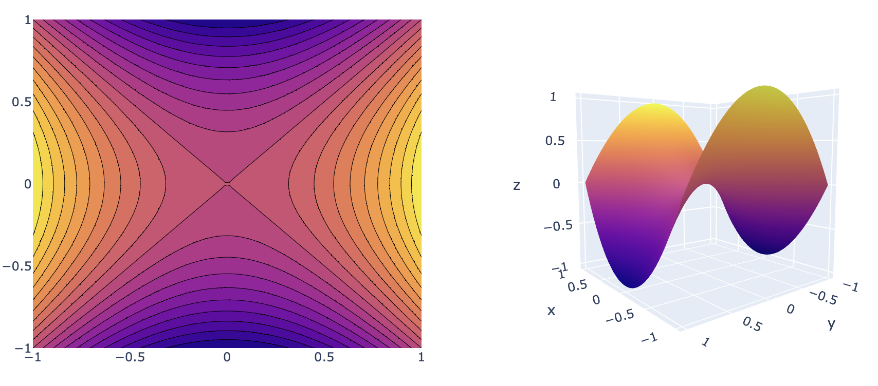
the fact that the Lagrangian function becomes stationary at the optimum
does not mean that this is a minimum. In fact, the stationary point of
the Lagrangian is a saddle point (see Figure 3.1), i.e. it is a minimum w.r.t. the
design variables and a maximum w.r.t. the Lagrange multipliers.
Figure 3.1: Example of the
contours and a 3D surface plot of a saddle point for \(\mathbf{x} \in
\mathcal{R}^2\).
One option to find the saddle point is called the primal
method, where the Lagrangian is first maximized w.r.t. \(\pmb{\mu}\) and \(\pmb{\lambda}\) with fixed \(\mathbf{x}\) and then minimized w.r.t.
\(\mathbf{x}\). Visually this is a
descent along the ridge until we reach the saddle point. This
formulation \[\min_{\mathbf{x} \in
\mathcal{X}} \underbrace{\max_{\pmb{\mu},\pmb{\lambda}}
\mathcal{L}(\pmb{\mu}, \pmb{\lambda},
\mathbf{x})}_{\bar{\mathcal{L}}(\mathbf{x})}{\qquad(3.49)}\] does
not provide much improvement, because the inner term \(\bar{\mathcal{L}}(\mathbf{x})\) just states
the constraints \[\begin{aligned}
\frac{\partial \mathcal{L}}{\partial \mu_i} &= g_i(\mathbf{x}) =
0 \quad i \in \mathcal{I}{\qquad(3.50)}\\
\frac{\partial \mathcal{L}}{\partial \lambda_j} &=
h_j(\mathbf{x}) = 0 \quad j \in [1,m]
{\qquad(3.51)}\end{aligned}\] with \(\mathcal{I}\) denoting the set of active
inequality constraints. This leaves us with the same problem as 3.1 and not much has been
gained.
However, it can be shown that for convex problems with linearly
independent inequality constraints, we can invert the process and
minimize the Lagrangian function w.r.t. \(\mathbf{x}\) first and then maximize it
w.r.t. \(\pmb{\mu}\) and \(\pmb{\lambda}\). Visually this is a
maximization along the valley floor until we reach the saddle point
(Harzheim 2014).
The formulation \[\max_{\pmb{\mu},\pmb{\lambda}}
\underbrace{\min_{\mathbf{x}\in \mathcal{X}} \mathcal{L}(\pmb{\mu},
\pmb{\lambda}, \mathbf{x})}_{\underline{\mathcal{L}} (\pmb{\mu},
\pmb{\lambda})}{\qquad(3.52)}\] is helpful, because we are left
with very simple box constraints in these optimization problems (\(\mathbf{x} \in \mathcal{X}\) in the inner
minimization and \(\pmb{\mu} \ge 0\) in
the maximization).
Example: Dual problem
We want to find the solution of the following quadratic optimization
problem for \(\mathbf{x} \in
\mathcal{R}^2\)\[\begin{aligned}
\min_{\mathbf{x}} \quad & f(\mathbf{x})=
(\mathbf{x}-\tilde{\mathbf{x}}) \cdot \mathbf{Q} \cdot
(\mathbf{x}-\tilde{\mathbf{x}}){\qquad(3.53)}\\
\textrm{s.t.} \quad & h(\mathbf{x}) = (x_1+1)^2 +
x_2 = 0 {\qquad(3.54)}\\
{\qquad(3.55)}\end{aligned}\] with \[\mathbf{Q} =
\begin{pmatrix}
2 & 0 \\
0 & 1
\end{pmatrix}
\quad
\text{and}
\quad
\tilde{\mathbf{x}} =
\begin{pmatrix}
-1\\
1
\end{pmatrix}.{\qquad(3.56)}\]
This is visually equivalent to searching for a point on the black
line in the following image that has the smallest function value.
We can formulate the Lagrangian function as \[\mathcal{L}(\mathbf{x}, \lambda) = 2
(x_1-\tilde{x}_1)^2 + (x_2-\tilde{x}_2)^2 + \lambda \left[(x_1+1)^2 +
x_2 \right].{\qquad(3.57)}\] Now, we solve the dual problem by
first minimizing the Lagrange function w.r.t. \(\mathbf{x}\). For the stationary point,
\[\begin{aligned}
\frac{\partial \mathcal{L}}{\partial x_1} &= 4 x^*_1 +4 + 2
\lambda x^*_1 + 2 \lambda = 0{\qquad(3.58)}\\
\frac{\partial \mathcal{L}}{\partial x_2} &= 2 x^*_2 - 2 +
\lambda = 0
{\qquad(3.59)}\end{aligned}\] applies. Hence, we can substitute
\[\begin{aligned}
x^*_1(\lambda) = -1 {\qquad(3.60)}\\
x^*_2(\lambda) = 1 - \frac{1}{2} \lambda
{\qquad(3.61)}\end{aligned}\] in \(\mathcal{L}\) to obtain the dual objective
function \(\underline{\mathcal{L}}
(\lambda)\). Now, we are left with a problem \[\max_{\lambda} \underline{\mathcal{L}} (\lambda)
=
\max_{\lambda} \left( - \frac{\lambda^2}{4} + \lambda
\right).{\qquad(3.62)}\] The maximum is located at a stationary
point, so with \[\frac{\partial
\underline{\mathcal{L}} }{\partial \lambda} = 1 - \frac{\lambda^*}{2} =
0{\qquad(3.63)}\] we get \(\lambda^*=2\), \(x_1^*=-1\) and \(x_2^*=0\).
The example shows that we need to be able to express the design
variables \(\mathbf{x}\) in terms of
the Lagrangian variables in order to apply the dual method. This is
typically not applicable to general optimization problems. However, the
dual method is very attractive for separable convex
optimization problems, i.e. if the objective function can be expressed
as \[f(\mathbf{x}) = f_0 + \sum_{k=1}^d
f_k(x_k){\qquad(3.64)}\] and the constraints can be expressed as
\[\begin{aligned}
g_i(\mathbf{x}) & = g_{i0} + \sum_{k=1}^d g_{ik}(x_k) \quad i
\in [1,n]{\qquad(3.65)}\\
h_j(\mathbf{x}) & = h_{j0} + \sum_{k=1}^d h_{jk}(x_k) \quad j
\in [1,m].
{\qquad(3.66)}\end{aligned}\] Then, the Lagrangian becomes \[\mathcal{L} (\mathbf{x}, \pmb{\mu},
\pmb{\lambda}) = f_0 + \sum_{k=1}^d f_k(x_k) + \sum_{i=1}^n \mu_i
\left(g_{i0} + \sum_{k=1}^d g_{ik}(x_k) \right) + \sum_{j=1}^m
\lambda_j \left(h_{j0} + \sum_{k=1}^d h_{jk}(x_k)
\right){\qquad(3.67)}\] and is also separable \[\mathcal{L} (\mathbf{x}, \pmb{\mu},
\pmb{\lambda}) = \mathcal{L}_0 + \sum_{k=1}^d
\mathcal{L}_k(x_k){\qquad(3.68)}\] with \[\begin{aligned}
\mathcal{L}_0 &= f_0 + \sum_{i=1}^n \mu_i g_{i0} + \sum_{j=1}^m
\lambda_j h_{j0} {\qquad(3.69)}\\
\mathcal{L}_k (x_k) & = f_k(x_k) + \sum_{i=1}^n \mu_i
g_{ik}(x_k) + \sum_{j=1}^m \lambda_j h_{jk}(x_k).
{\qquad(3.70)}\end{aligned}\] For such a separable convex
problem, the search for the the "valley floor" \[\min_{\mathbf{x}\in \mathcal{X}}
\mathcal{L}(\pmb{\mu}, \pmb{\lambda}, \mathbf{x}){\qquad(3.71)}\]
turns into \(d\) simple strictly convex
optimization problems \[\min_{x_k \in [x_k^-,
x_k^+]} \mathcal{L}_k(x_k) \quad k \in[1,d]{\qquad(3.72)}\] which
have a unique solution and are simple to solve because each of them is
just a box-constrained single variable optimization problem. After
finding the expression for \(\underline{\mathcal{L}} (\pmb{\mu},
\pmb{\lambda})\) easily, we only need to solve this remaining
problem \(\max_{\pmb{\mu}, \pmb{\lambda}}
\underline{\mathcal{L}} (\pmb{\mu}, \pmb{\lambda})\) w.r.t. \(\pmb{\mu}\) and \(\pmb{\lambda}\). The dual problem is
therefore especially well suited for separable convex problems with
\(d \gg n+m\), i.e. for problems with
many design variables and just a few constraints. This is typically the
case for topology optimization.
Example: Separable problem
Let’s consider the previous example with the additional constraint \(\mathbf{x} \in \mathcal{X} = [0, 2]\times[-2,
2]\). This is visually equivalent to searching within the gray
box for a point on the black line that has the smallest function value
in the following image.
It would be tedious to solve the problem with additional inequality
constraints like \(g_1= x_1, g_2=x_1-2,
g_3=x_2-2, g_4=2-x_2\).
However, we can formulate a separable Lagrangian function as \[\mathcal{L}(\mathbf{x}, \lambda) = \underbrace{2
(x_1-\tilde{x}_1)^2 + \lambda (x_1+1)^2}_{\mathcal{L}_1(x_1)} +
\underbrace{(x_2-\tilde{x}_2)^2 + \lambda
x_2}_{\mathcal{L}_2(x_2)}.{\qquad(3.73)}\] and can take care of
box constraints trivially in each optimization by clamping. Using the
stationary points \[\begin{aligned}
\frac{\partial \mathcal{L}_1}{\partial x_1} &=
4\hat{x}_1+4+2\lambda \hat{x}_1 + 2 \lambda = 0 {\qquad(3.74)}\\
\frac{\partial \mathcal{L}_2}{\partial x_2} &=
2\hat{x}_2-2+\lambda = 0
{\qquad(3.75)}\end{aligned}\] we can solve \[\begin{aligned}
x_1^*(\lambda) = \textrm{clamp}(\hat{x}_1(\lambda), x_1^-,
x_1^+) &= 0 {\qquad(3.76)}\\
x_2^*(\lambda) = \textrm{clamp}(\hat{x}_2(\lambda), x_2^-,
x_2^+) &=
\begin{cases}
2 & \quad \lambda < -2 \\
-2 & \quad \lambda > 6 \\
1 - \frac{\lambda}{2} & \quad \text{else}
\end{cases}
{\qquad(3.77)}\end{aligned}\] and the dual objective function
becomes \[\underline{\mathcal{L}}(\lambda) =
\begin{cases}
3 + 3 \lambda & \quad \lambda < -2 \\
11 - \lambda & \quad \lambda > 6 \\
2 + 2 \lambda - \frac{\lambda^2}{4} & \quad
\text{else.}
\end{cases}{\qquad(3.78)}\] This dual objective function
is plotted here:
We can employ any gradient descent method or analytical method to
find the optimum of the dual function. In this case, it is \(\lambda^*=4\) and therefore the optimum is
at \(x_1^*=0\) and \(x_2^*=-1\).
References
Christensen, Peter W., and Anders Klarbring. 2008. An Introduction to Structural Optimization.
Springer Netherlands.
Harzheim, Lothar. 2014. Strukturoptimierung,
Grundlagen und Anwendungen. Europa Lehrmittle.
Karush, William. 1939. “Minima of Functions
of Several Variables with Inequalities as Side
Conditions.”
Kuhn, H. W., and A. W. Tucker. 1951. “Nonlinear
Programming.”Proceedings of the Second Berkeley
Symposium on Mathematical Statistics and Probability 2: 481–92.